
 Add as preferred on Google

The Best LLMs in 2026: A Comparison and What to Expect in 2027Read More

AI model compression reduces the storage, memory traffic, or computation required to run a trained model, with an acceptable change in task quality. The main techniques are pruning, quantization, knowledge distillation, low-rank factorization, sparse attention, and adaptive computation. Their results depend on the architecture, dataset, inference hardware, and accuracy requirements.
A model with fewer parameters can still respond slowly. A model stored in 4-bit weights can still require substantial memory for activations and the key-value cache. The practical goal is to measure what a system gains from compression, then check what it gives up.
The history of neural networks explains how we reached this point. Each architectural advance helped machines recognize another kind of pattern. Each advance also introduced costs that later research had to address.
Early humans improved a spear-thrower's range through a longer lever. The physical principle was available long before anyone expressed mechanical advantage mathematically. Small design changes made a difficult task easier. Similar observations appear in nature, from selective neural activity to the way organisms allocate limited energy.
These parallels are useful for understanding the motivation behind model compression. Biological systems and artificial neural networks have different mechanisms, so an analogy should remain an analogy. Still, both have to work within physical constraints.
Claude Shannon's information theory gave us one mathematical way to describe uncertainty:
H(X) = −Σ p(x) log₂ p(x)
Here, p(x) is the probability of an outcome. Entropy measures expected information or uncertainty in a distribution. It does not directly measure how many model weights can be removed. Compression research builds on related ideas about redundancy, information representation, and acceptable distortion.
Frank Rosenblatt's perceptron supplied a simple learning rule:
w_new = w_old + η(target − output)x
The learning rate η controls the update size, and x is the input associated with the weight. We can already see the idea that runs through the series: useful behavior depends on how connections are adjusted and represented.

An artificial neuron combines weighted inputs with a bias, then applies an activation function:
z = Σ(wᵢxᵢ) + b
a = f(z)
Activation functions determine how these signals propagate. Three common choices illustrate the design space:
Training adjusts the parameter vector θ to reduce a loss function. Mean squared error is often used in regression. Cross-entropy is common in classification:
MSE = (1/N) Σ(y_pred − y_true)²
Cross-entropy = −Σ y_true log(y_pred)
Gradient descent follows the direction of decreasing loss:
θ_new = θ_old − η∇L(θ)
For a particular weight, backpropagation applies the chain rule:
∂L/∂wᵢ = (∂L/∂a)(∂a/∂z)(∂z/∂wᵢ)
This creates two practical concerns. If a learning rate is too large, updates can oscillate or diverge. If derivatives repeatedly shrink as they pass through layers, early parameters receive little useful training signal. Increasing depth also grows activation memory and compute requirements. The later history of neural architectures follows the effort to represent richer information without losing the ability to train or deploy the network efficiently.
A feedforward network processes an input according to its current activations. Sequential problems require a representation of what happened before. The meaning of a word, for example, often depends on earlier words in the sentence.
A recurrent neural network (RNN) carries a hidden state between steps:
hₜ = tanh(Wₕₕhₜ₋₁ + Wₓₕxₜ + bₕ)
The current state hₜ combines the new input xₜ with the previous hidden state hₜ₋₁. This gives the network a mechanism for sequence context. Backpropagation through time must multiply many Jacobians, which can cause gradients to decay or grow. That is why early RNNs often struggled with long-distance dependencies.

Long Short-Term Memory networks, introduced by Sepp Hochreiter and Jürgen Schmidhuber in 1997, introduced a cell state and gates that control information flow. In a simplified modern LSTM formulation:
iₜ = σ(Wᵢ[hₜ₋₁, xₜ] + bᵢ)
fₜ = σ(Wf[hₜ₋₁, xₜ] + bf)
gₜ = tanh(Wg[hₜ₋₁, xₜ] + bg)
cₜ = fₜ ⊙ cₜ₋₁ + iₜ ⊙ gₜ
oₜ = σ(Wo[hₜ₋₁, xₜ] + bo)
hₜ = oₜ ⊙ tanh(cₜ)
Here, iₜ decides how much candidate information enters memory, fₜ controls retained state, and oₜ selects what becomes visible in the hidden output. The elementwise multiplication operator is ⊙.
A mystery novel provides a useful analogy. A reader keeps track of a suspect, discards an irrelevant clue, then recalls an earlier event when new evidence appears. LSTM gates approximate these selective updates through learned numerical functions. The additional gates have a cost in parameters and sequential computation, which matters when choosing an architecture for a resource-limited application.
Vision introduced a different problem. An image contains many local patterns, and their arrangement matters. Convolutional neural networks (CNNs) apply shared filters across spatial locations, allowing one kernel to detect a similar feature in different parts of an image.
A discrete 2D convolution can be expressed as:
(I * K)[i,j] = ΣₘΣₙ I[i−m, j−n]K[m,n]
Deep-learning libraries commonly implement cross-correlation, which uses the kernel without reversing its indices. The familiar sliding-filter explanation applies to both operations.
For example, an edge detector may use the kernel:
[-1  0  1]
[-2  0  2]
[-1  0  1]
The filter responds to changes in pixel intensity across the image. Early CNN layers can learn edges and textures, with deeper layers building representations of larger features and objects.

Pooling reduces the spatial resolution of feature maps. A 2×2 max-pooling operation on [[2.1, 1.4], [0.8, 1.9]] returns 2.1. Pooling can reduce downstream computation and provide some local translation tolerance. The selected architecture determines how much spatial detail remains available.
Weight sharing already makes CNNs efficient compared with a fully connected layer over the same image. Yet high-resolution feature maps and many channels still consume memory. Channel pruning, smaller kernels, quantization, and architecture-aware choices can reduce these costs.
Recurrent models process time steps in sequence. Attention makes it possible to compare a query with multiple positions and use the resulting relevance scores to combine information. In scaled dot-product attention:
Attention(Q, K, V) = softmax(QKᵀ/√dₖ)V
The query matrix Q represents what is being sought, K supplies matching features, and V contains the information to aggregate. Scaling by √dₖ helps control the size of dot products before softmax. Softmax converts scores into weights that sum to one along the attended dimension:
softmax(zᵢ) = e^zᵢ / Σⱼe^zⱼ

Transformers introduced multi-head attention, allowing several learned projections to examine relationships in parallel:
headᵢ = Attention(QWᵢQ, KWᵢK, VWᵢV)
MultiHead(Q,K,V) = Concat(head₁, ..., headₕ)Wo

Self-attention alone has no built-in ordering of tokens. The original transformer used sinusoidal positional encodings, including:
PE(pos,2i) = sin(pos/10000^(2i/d_model))
PE(pos,2i+1) = cos(pos/10000^(2i/d_model))

Full attention creates an n × n score matrix for a sequence of length n, giving quadratic attention-score size and pairwise interaction count in the usual implementation. FlashAttention-style kernels can reduce memory traffic and avoid materializing that full matrix, although dense attention retains its pairwise arithmetic. Sparse and windowed patterns reduce the number of interactions themselves.

Compression methods target different costs. The table is a starting point for choosing a technique, followed by the mathematics and practical examples.
| Method | Primary change | Main measurement | Typical constraint |
|---|---|---|---|
| Pruning | Removes weights, channels, or blocks | Sparsity, latency, task score | Sparse kernels and shape compatibility |
| Quantization | Reduces numerical bit width | Weight bytes, memory bandwidth, task score | Hardware support and outlier sensitivity |
| Knowledge distillation | Trains a smaller student | Student latency and quality | Teacher quality and training data |
| Low-rank factorization | Replaces a matrix with narrow factors | Parameter count, compute | Approximation error and rank |
| Sparse attention | Limits attended token pairs | Context compute and memory | Lost distant dependencies |
| Adaptive computation | Varies executed work per input | Average and tail latency | Routing overhead and calibration |
Magnitude pruning removes weights whose absolute value falls below a threshold τ:
w′ = 0 if |w| < τ; otherwise w′ = w
Consider the 5×5 matrix from the original compression example:
Before                         After threshold τ = 0.1
0.021 0.891 0.033 0.002 0.763   0     0.891 0     0     0.763
0.001 0.442 0.004 0.921 0.003   0     0.442 0     0.921 0
0.002 0.004 0.783 0.001 0.002   0     0     0.783 0     0
0.891 0.002 0.001 0.663 0.004   0.891 0     0     0.663 0
0.003 0.001 0.892 0.002 0.445   0     0     0.892 0     0.445
With input [0.5, 0.3, 0.8, 0.2, 0.7], the first row produces 0.8387 before pruning and 0.8014 after pruning. The difference is 0.0373, or approximately 4.4% of the original activation. The calculation concerns one neuron's activation. It gives no estimate of dataset-level classification accuracy. After pruning, fine-tuning and dataset-level evaluation determine whether the model retains useful performance.

Unstructured sparsity often needs specialized storage or kernels to improve runtime. Structured pruning removes whole channels, attention heads, or blocks, making speedups easier to realize on conventional accelerators. Sparse weights stored as zeros inside dense tensors may save little inference time.
A 32-bit floating-point weight requires four bytes. An 8-bit integer weight uses one byte before metadata and packing overhead, so the theoretical weight-storage reduction is 75%. This figure says nothing by itself about accuracy or inference latency.
For uniform affine quantization over a range [x_min, x_max] into unsigned 8-bit values:
q = round((x − x_min) × 255/(x_max − x_min))
x̂ = x_min + q(x_max − x_min)/255
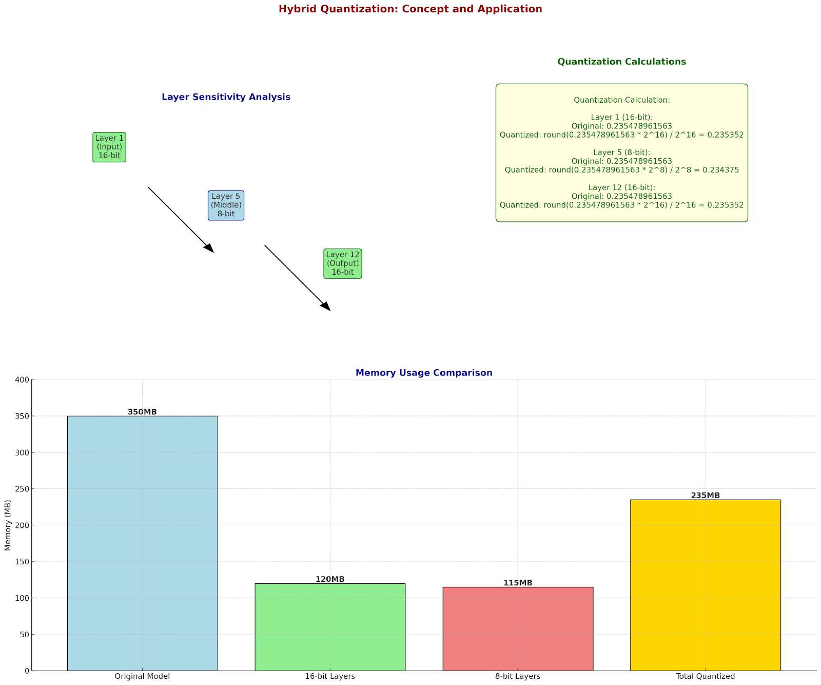
Taking x = 0.235478961563 and [−1, 1] gives q = 158, then x̂ ≈ 0.2392157. Quantization introduces a small numerical error for this value. Outliers, activation distributions, and accumulated layer errors must be measured across the complete model.
There are two common deployment paths. Post-training quantization (PTQ) converts a trained model using calibration or statistical information. Quantization-aware training (QAT) simulates low-precision effects during training and often uses a straight-through estimator to approximate gradients through rounding operations.

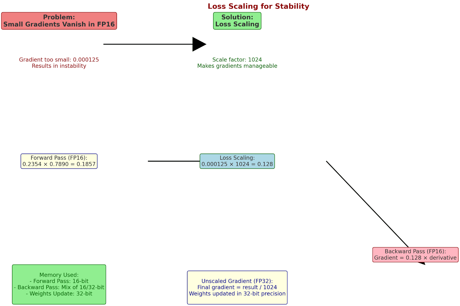
Mixed precision can preserve more bits in sensitive layers and fewer bits elsewhere. FP16 or BF16 training may improve throughput on supported accelerators, but training still needs appropriate accumulator precision and stability controls. With FP16, loss scaling can multiply a loss by 1024 during backpropagation and divide its gradients by 1024 before the optimizer update. This helps prevent small gradients from underflowing, although BF16 generally has a wider exponent range and often requires less intervention.
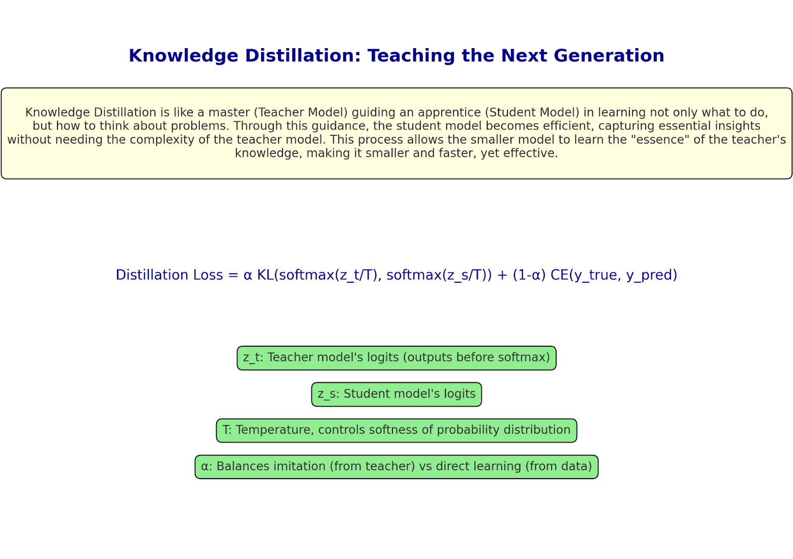
A large model can guide a smaller model by supplying a distribution over possible outputs. This exposes relationships between classes that hard labels do not express. Temperature T softens both teacher and student distributions:
p_teacher = softmax(z_teacher/T)
p_student = softmax(z_student/T)
A common objective combines a supervised cross-entropy loss with a distillation term:
L = (1−α) CE(y, p_student at T=1) + αT² KL(p_teacher || p_student)
The factor T² is a common convention for balancing gradients. The exact loss and weighting depend on the task. In the original series, a teacher passes a shorter network some of its learned behavior, much like an experienced researcher walking a student through the reasoning behind an answer.
A weight matrix W ∈ R^(m×n) may be approximated using lower-rank factors A ∈ R^(m×r) and B ∈ R^(r×n):
W ≈ AB, where r < min(m,n)
The parameter count changes from mn to r(m+n). For a 6×6 matrix and rank 2, a two-factor representation requires 24 parameters instead of 36, a one-third reduction. An explicit truncated singular-value decomposition can store U₂ (6×2), Σ₂ (2 singular values), and V₂ᵀ (2×6), requiring 26 scalars, a reduction of about 28%. Factoring the singular values into either side removes the need for a separate diagonal array.
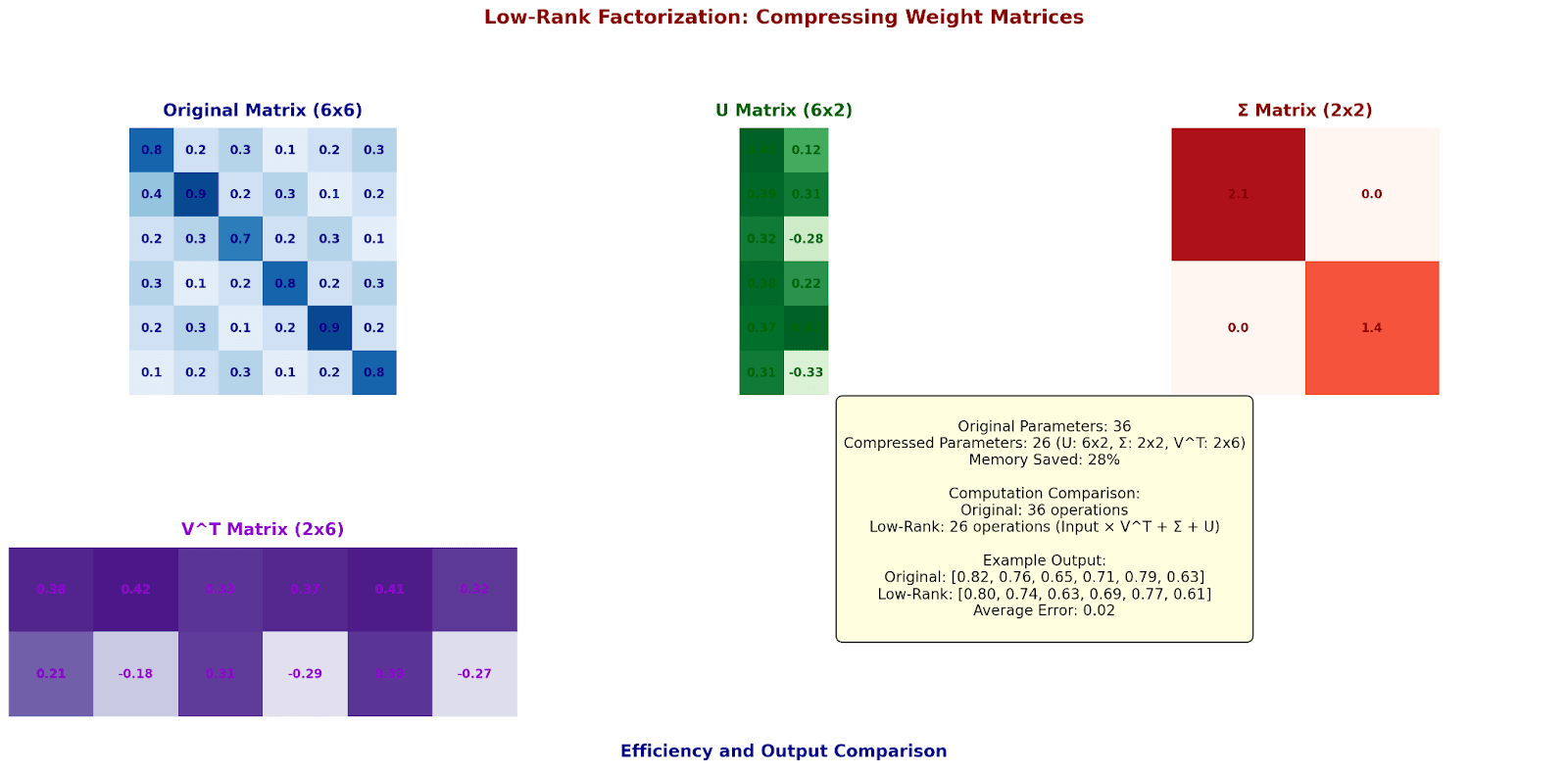
Low-rank compression changes the deployed weight representation. LoRA, a related adaptation technique, keeps a base weight frozen and learns a small low-rank update. Its principal saving is in trainable parameters during fine-tuning. Deploying the original base model still has a storage cost.
For eight tokens, dense self-attention evaluates up to 8 × 8 = 64 query-key pairs per head. A fixed window of four positions evaluates around 8 × 4 = 32, subject to boundary and masking rules. The example gives a 50% reduction in pairwise scores. The full runtime gain depends on the attention implementation and overheads. Windowing also restricts long-range interactions unless the architecture adds global or other connections.
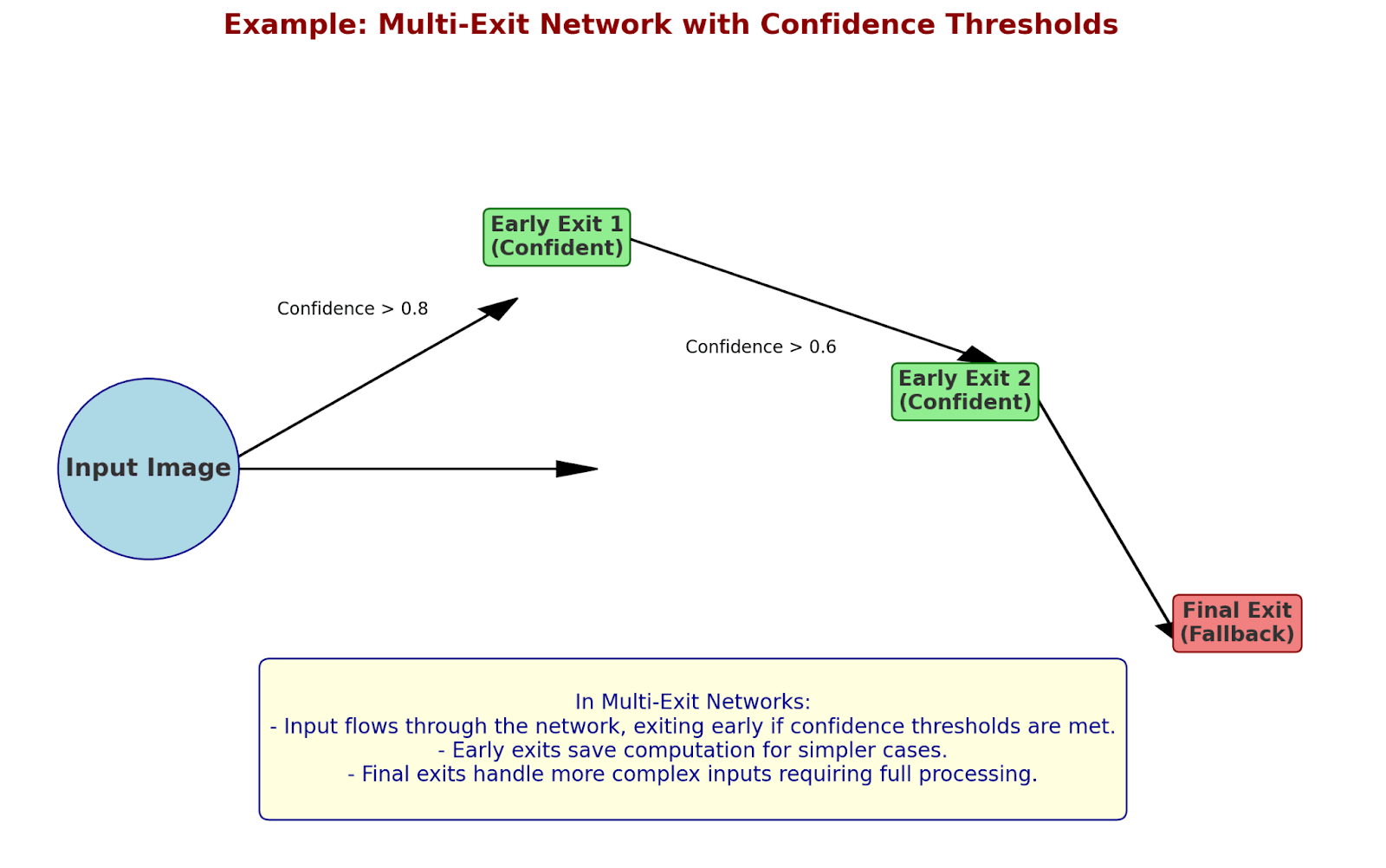
Adaptive computation takes a different route. An early-exit model may stop after nine layers when its output confidence exceeds a calibrated threshold. Harder examples may continue through all 24 layers. For one example exiting after nine layers, (24−9)/24 = 62.5% of those layer executions are skipped. Average savings require measurement across a representative workload; confidence is not automatically a reliable measure of correctness.
Conditional computation also appears in mixture-of-experts (MoE) networks, a topic explored in Ateeb Taseer's later writing on DeepSeek. A router selects a subset of specialist feedforward blocks for each token. This reduces the number of active parameters used in that pass, though the complete expert set must still be stored or distributed across devices. Routing imbalance and communication can erase expected throughput gains. A useful evaluation separates total parameters, active parameters per token, weight storage, and observed inference cost.
For generative transformers, the key-value (KV) cache deserves separate attention. It grows with retained sequence length, layers, heads, and per-element precision. Weight-only INT8 or 4-bit compression may leave this cache largely unchanged. KV-cache quantization, grouped-query attention, or context-management strategies can address it, each with its own quality and implementation constraints.
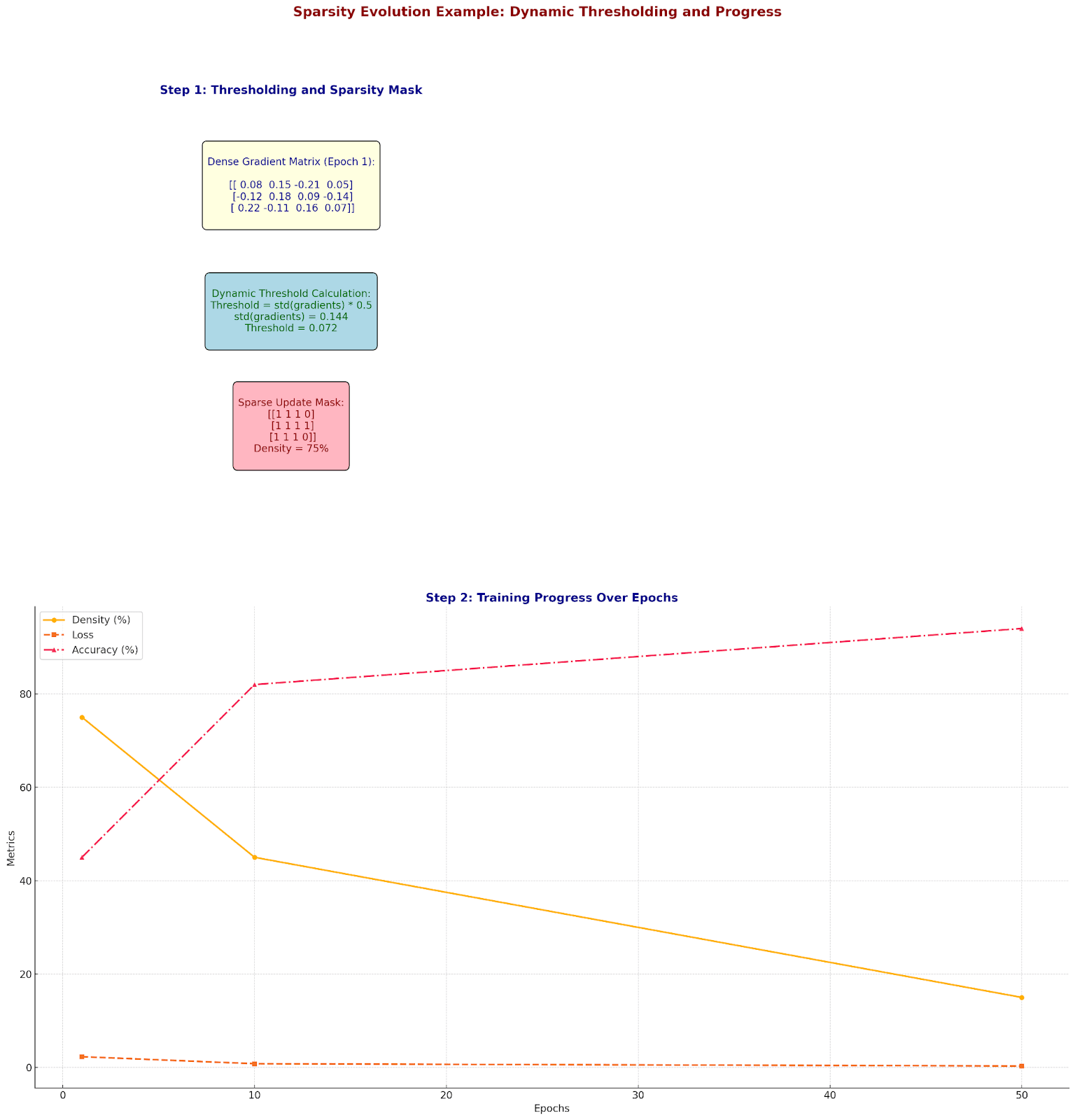
Dynamic sparse training extends selective computation into the training process. Connections may be removed and regrown according to importance estimates, gradient signals, or an allocated sparsity budget. The resulting accuracy and energy usage must be validated experimentally.
A layer with 1024 inputs and 1024 outputs contains 1,048,576 weights. FP32 weight storage is 4 MiB. INT8 weight storage is 1 MiB, excluding scales and alignment. If inference repeatedly fetches those weights from slow memory, lower precision can save bandwidth. If the compute kernel lacks an efficient INT8 path, the observed speed improvement may be small or even negative.
Convolutions have another opportunity: data reuse. A 3×3 convolution with 256 input channels and 256 output channels has 589,824 weights. An activation map measuring 56×56×256 has 802,816 values. In a naive accounting of FP32 storage, those are approximately 2.25 MiB of weights and 3.06 MiB per activation map. Tiling the output into 14×14 regions allows a kernel to reuse patches and weights through on-chip memory. The amount of external-memory traffic saved depends on cache capacity, layout, fusion, and the implementation.
Hardware-aware architecture search uses measured latency or device constraints as part of the model selection process. A search objective might include a quality penalty and explicit memory or latency costs:
J = L_task + λ_latency C_latency + λ_memory C_memory
This makes deployment constraints part of optimization. The coefficients need calibration against actual requirements; a theoretical FLOP estimate cannot substitute for latency measurements.
A dynamic sparse training method updates its connection mask during learning. One illustrative rule uses τ = 0.5 × std(gradients) and suppresses updates whose gradient magnitude falls below τ. More advanced methods periodically regrow promising connections to maintain a useful sparsity pattern. The source series shows a hypothetical training trajectory in which density changes from 75% to 15%. Those values should be treated as an example of the mechanism, not a reproducible accuracy benchmark.
Energy-aware compression models the work completed by the device and the cost of moving data:
E_total ≈ N_compute e_compute + N_memory e_memory + E_overhead
Here, N counts operations or memory accesses, e is their estimated energy per operation, and overhead includes runtime and device effects. For a purely illustrative calculation, 1,048,576 operations at 3.7 pJ each plus 2,048 accesses at 340 pJ each equal approximately 4.58 μJ. The original series labels the same numerical total in millijoules; microjoules are the correct units for those assumptions. Real energy figures vary significantly between devices, memory levels, and operating conditions.
A battery-powered model might choose a lower precision or a shallower execution path when its power budget tightens. The system still needs to check accuracy and latency after the switch. Dynamic decisions add control overhead and can make tail latency harder to predict.
Compression generally works best when its stages are evaluated together. Consider the illustrative model trajectory in the original series:
| Stage | Parameter count | FP32 or INT8 weight storage, excluding overhead |
|---|---|---|
| Original teacher, 12 layers | 125 million | 500 MB at FP32 |
| Distilled student, 8 layers | 84 million | 336 MB at FP32 |
| Narrower student, 8 layers | 37 million | 148 MB at FP32 |
| Same narrower student, INT8 | 37 million | 37 MB at INT8 |
The last model has approximately 92.6% fewer raw weight bytes than the first. These are arithmetic examples using the supplied parameter counts, not benchmark results. Actual checkpoints include metadata and other tensors. Running the model also requires activations, temporary buffers, and hardware-specific runtime memory.

A sensible workflow starts with a stable baseline. Measure held-out quality, peak memory, throughput, p50 and p95 latency, and energy per inference on the intended hardware. Identify whether the bottleneck comes from weights, activations, attention, memory bandwidth, or unsupported operators. Choose a suitable compression method, retrain or calibrate as needed, then compare at the same batch size and sequence length. Record any regression for important user groups or difficult inputs.
Hardware-aware optimization may include tiling, kernel fusion, structured sparsity, and choosing quantization formats with supported kernels. A smaller theoretical operation count does not guarantee lower latency. Memory transfers can dominate energy use, so a change that improves data locality may matter more than a change that saves arithmetic.
The human brain runs on roughly 20 watts, a striking reminder that intelligence operates under an energy budget. Comparing its operations per second directly with those of a GPU is difficult because biological spikes and floating-point arithmetic are different units of computation. Claims about a precise year when biological and artificial systems will converge should therefore remain speculative.
Neuromorphic hardware, conditional execution, improved memory systems, and low-precision arithmetic give researchers several ways to reduce energy use. Some approaches make an existing model smaller. Others change which parts of a model execute or how data moves through the chip. All face the same engineering requirement: demonstrate a useful quality-efficiency trade-off for the application.
For an edge vision system, the best outcome may be a model that fits within an 8 GB memory budget and processes an image within a latency limit. For a language model, context length and KV-cache growth may drive the decision. In either case, compression has succeeded when measured performance remains suitable for the real task at a lower resource cost.
Pruning removes selected weights or structural components. Quantization stores or computes values at lower precision. They can be combined, but each requires its own measurement of quality and hardware performance.
Sometimes. Models may contain redundancy that can be removed with little measurable impact on a defined benchmark. There is no general guarantee. The outcome depends on compression strength, fine-tuning, data distribution, and how accuracy is measured.
Weight quantization is often a practical starting point for reducing model memory. Distillation is useful when a smaller architecture is available and training data can support it. Sparse or efficient attention addresses context processing, and hardware-aware choices decide whether theoretical savings appear in production.
No fixed relationship holds across devices and workloads. Energy depends on hardware utilization, memory access, execution time, operator implementation, and batch size. Measurements on the target system are necessary.
Use the same held-out task data for baseline and compressed models, including difficult cases. Report accuracy or task quality together with weight storage, total peak memory, latency distributions, throughput, and energy on named hardware. State precision and sequence length so the comparison can be reproduced.
...Loading Related Blogs
Trusted by top platforms for our transformative solutions and exceptional results: