AI Model Compression Part VIII: The Compression Revolution - Finding Power in Simplicity

The Resource Crisis

By 2022, training a single large language model could consume more energy than 100 American households use in a year. This crisis echoed an ancient pattern: every complex system eventually faces the limits of its resources. Just as ancient civilizations had to optimize their resource usage or collapse, AI faced its own moment of reckoning.

The Fundamental Trade-off

Model Capability vs Resource Usage: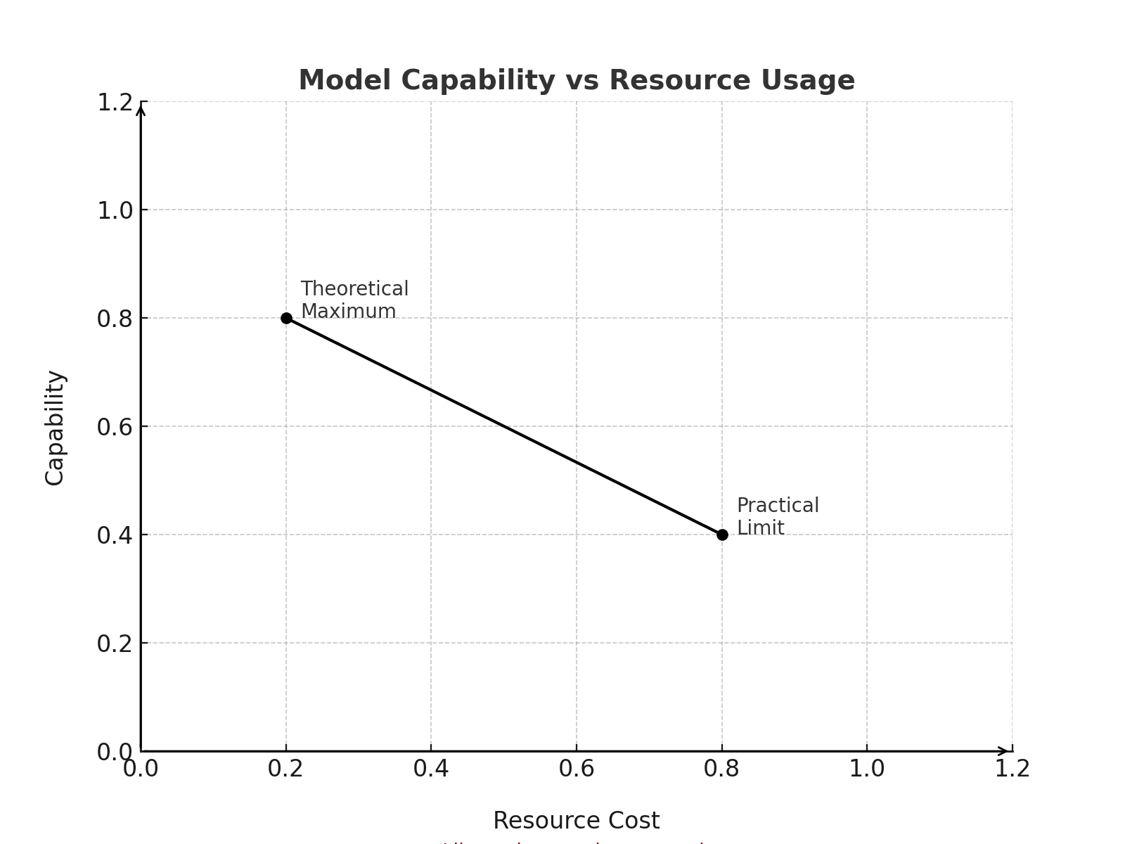

Like a city growing upward: at some point,

the cost of adding each new floor outweighs its benefits.

The Mathematics of Less is More

Pruning: The Art of Selective Forgetting

Nature had already solved this problem. During adolescence, human brains undergo synaptic pruning, removing unused connections to optimize neural pathways. AI researchers took inspiration from this biological process:

Magnitude-based Pruning:

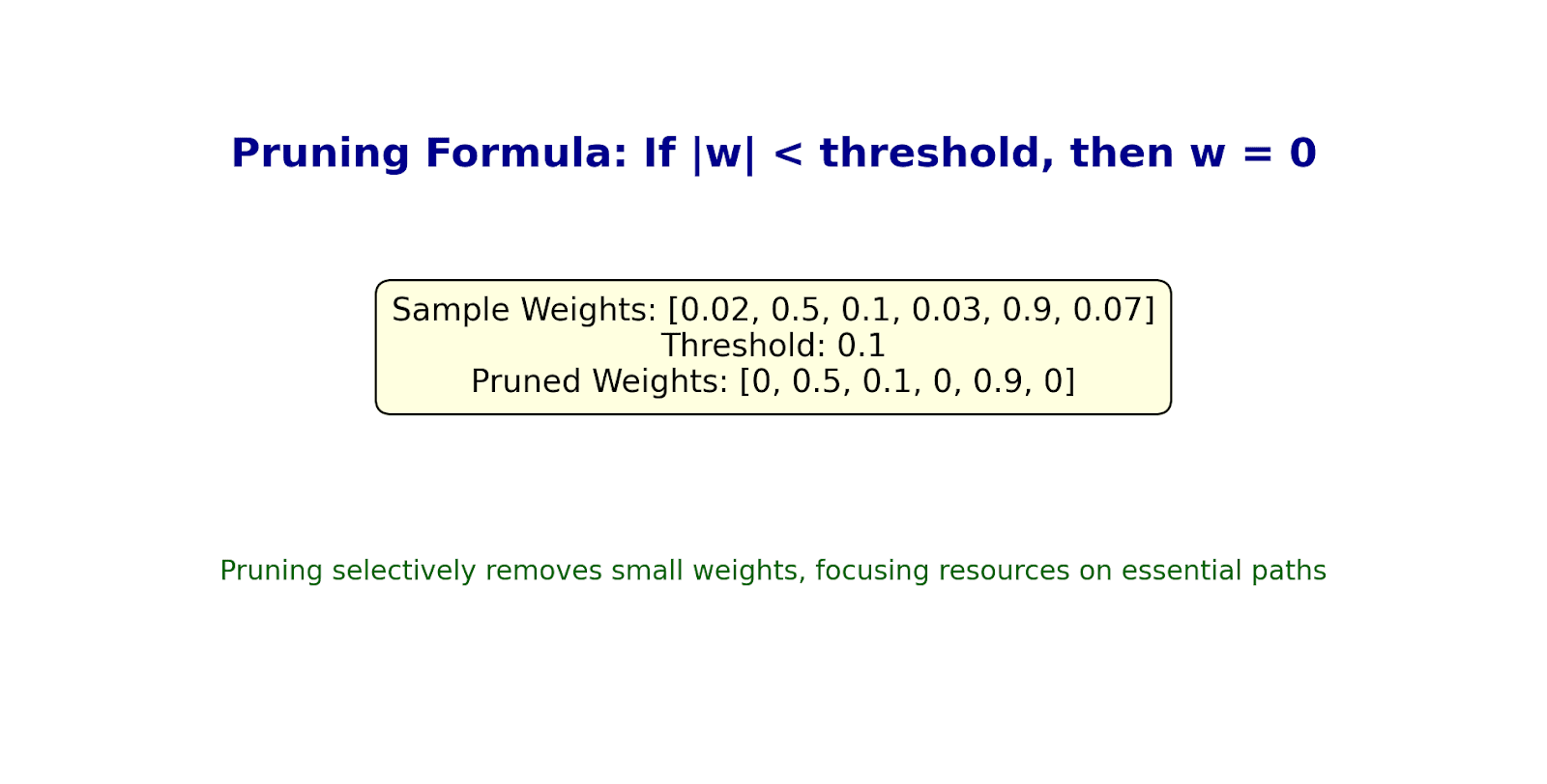
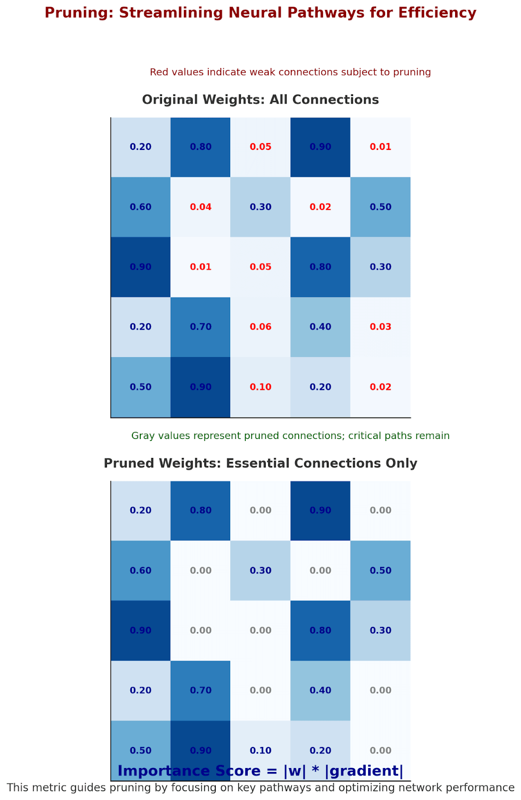
Like a gardener pruning a tree:

• Small, weak branches are removed
• Strong, essential pathways remain
• The tree grows more efficiently

But the real insight came in understanding which connections to keep. The mathematics tells a beautiful story:

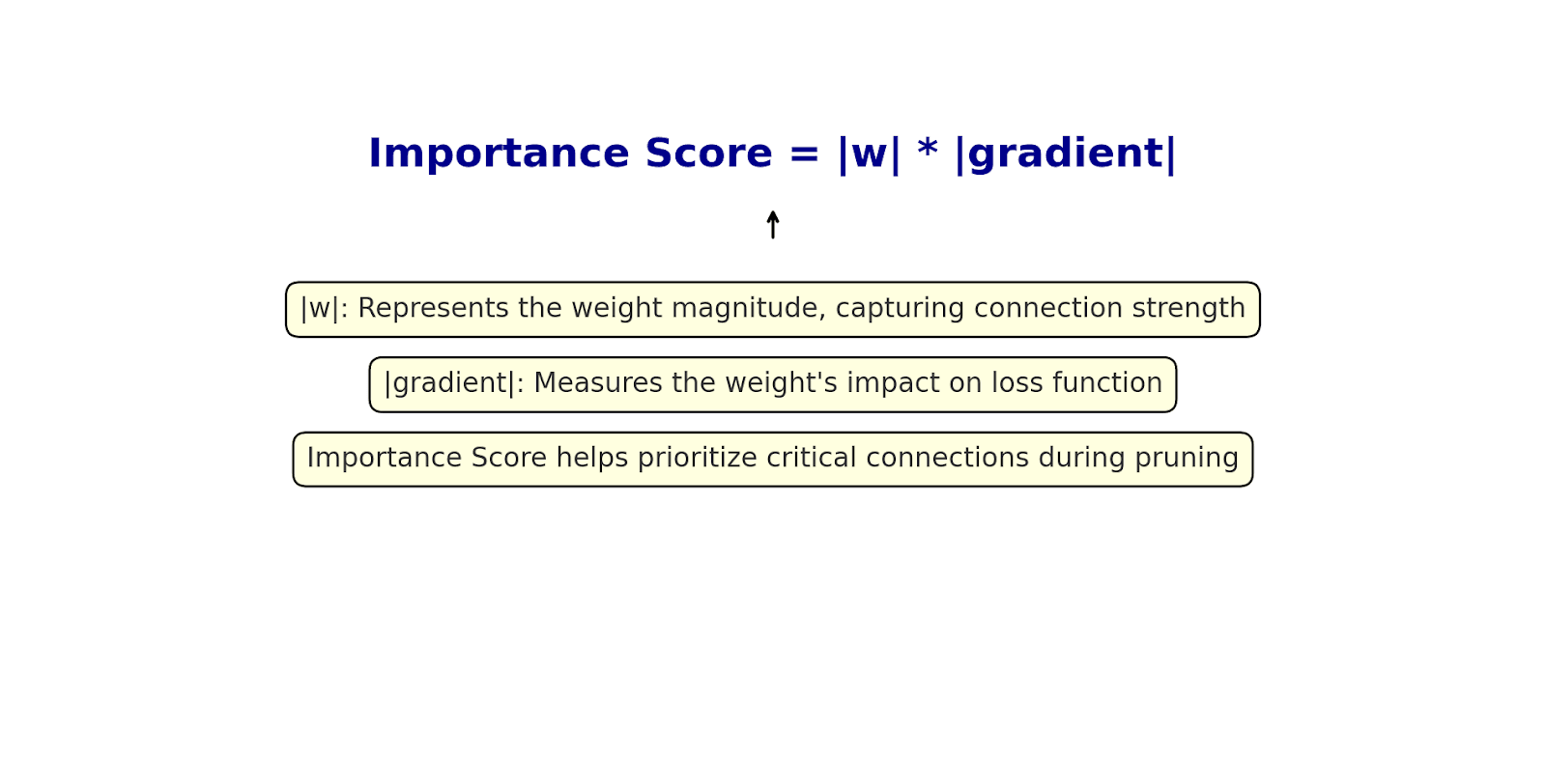
This mirrors how our brain strengthens frequently used neural pathways while letting unused ones fade.

Quantization: The Poetry of Precision

Traditional neural networks used 32-bit floating-point numbers for weights, like using a dictionary to spell "cat." Quantization showed we could use much less:

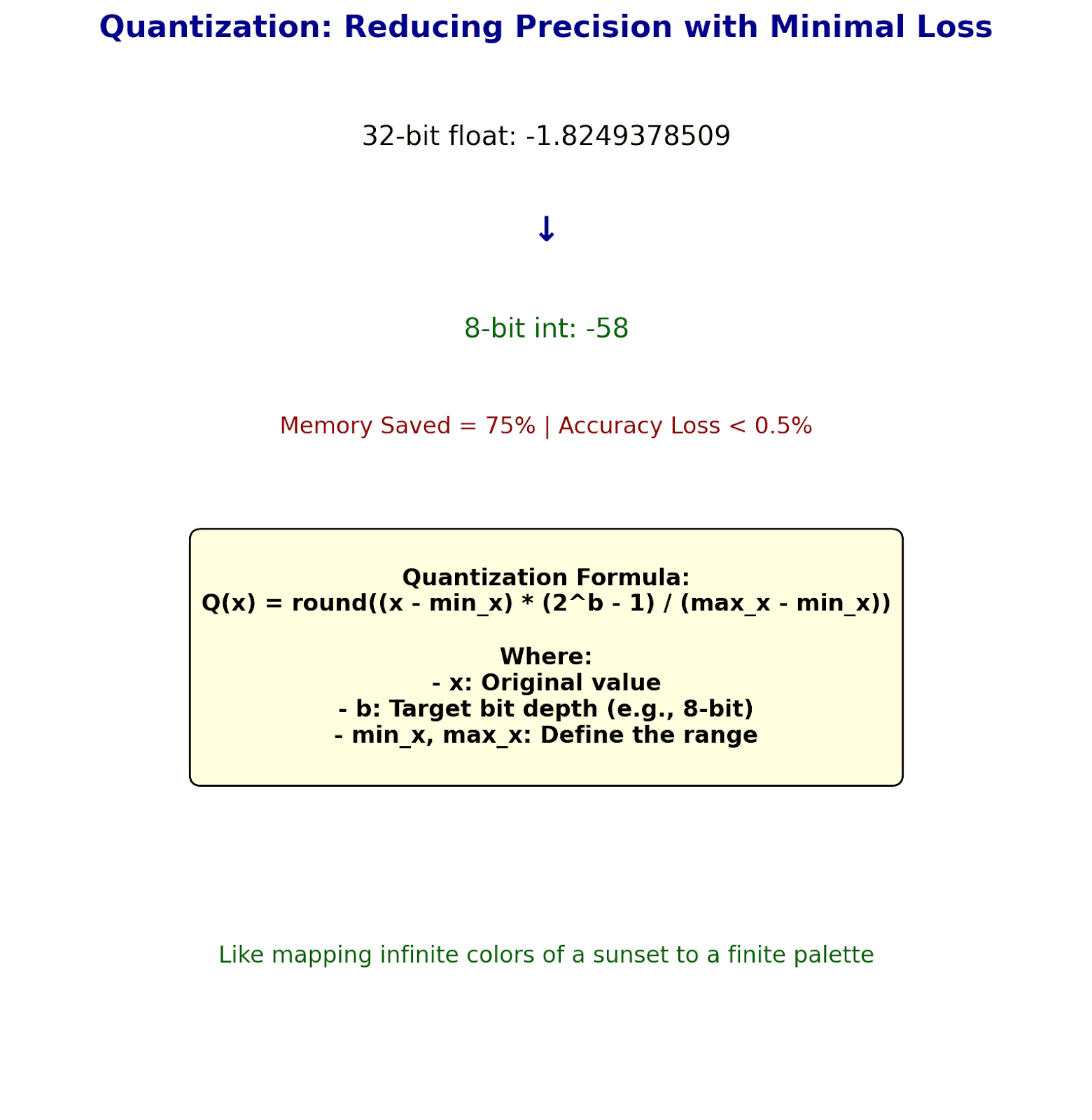
Like human language evolution: We don't need infinite precision to communicate meaning.

The mathematics of quantization tells a story of elegant approximation:

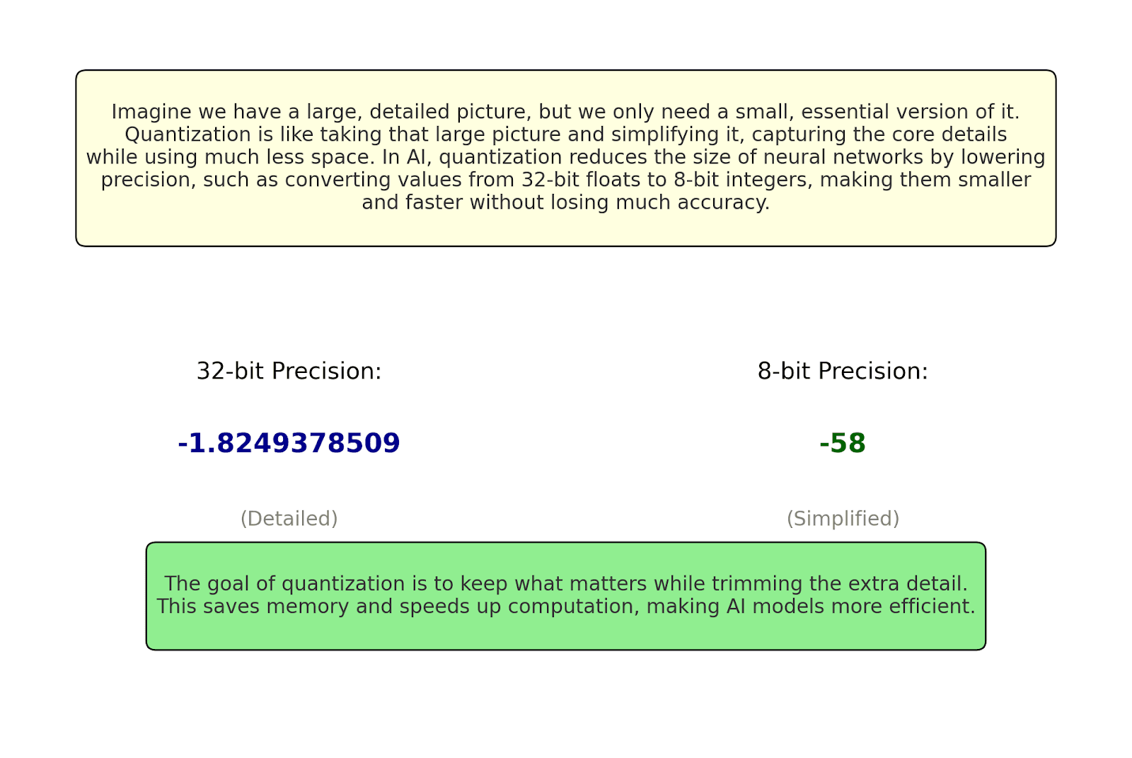
This is like mapping the infinite colors of a sunset into a finite but beautiful palette.

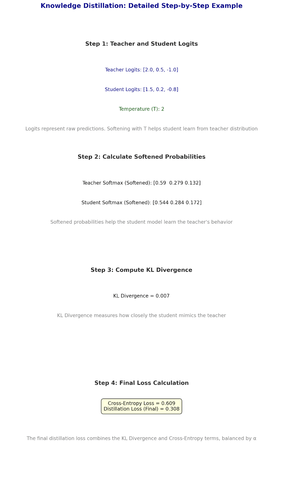
Knowledge Distillation: Teaching the Next Generation

Perhaps the most profound compression technique mirrors how human knowledge passes through generations. A larger "teacher" model guides a smaller "student":

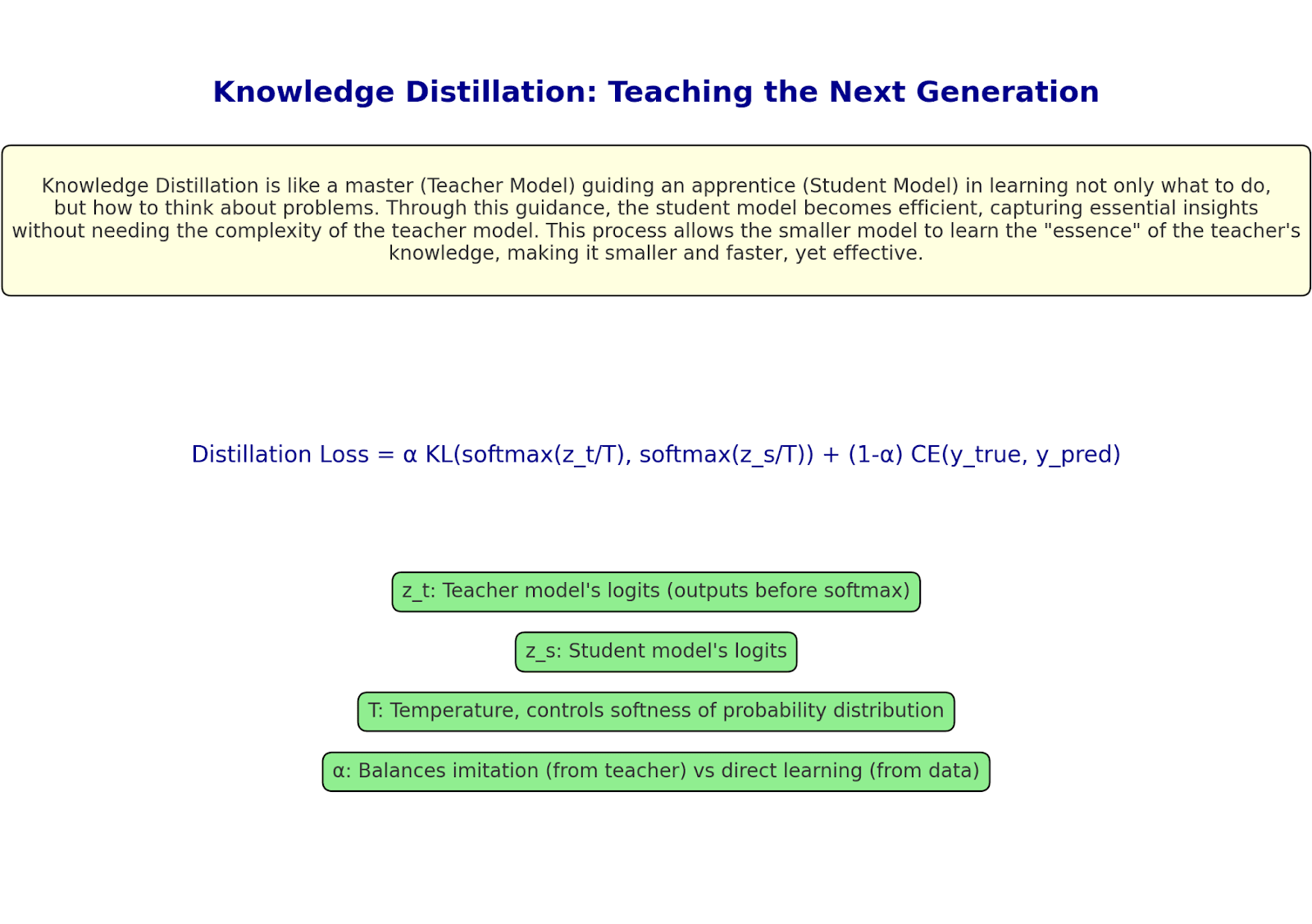
Like a master teaching an apprentice:

• The student learns not just the what, but the how
• Subtle patterns transfer through example
• The apprentice becomes efficient through guidance

The Modern Compression Symphony

Low-Rank Approximation: Finding Hidden Patterns

Consider how our brain compresses memories, we don't store every detail, but rather the essential patterns. Low-rank approximation does the same:

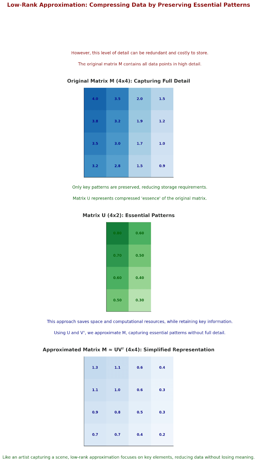
Like an artist capturing a landscape: They don't paint every leaf, but rather the essential patterns that create the scene.

The Emergence of Adaptive Computation

The latest revolution comes in models that adapt their complexity to the task:

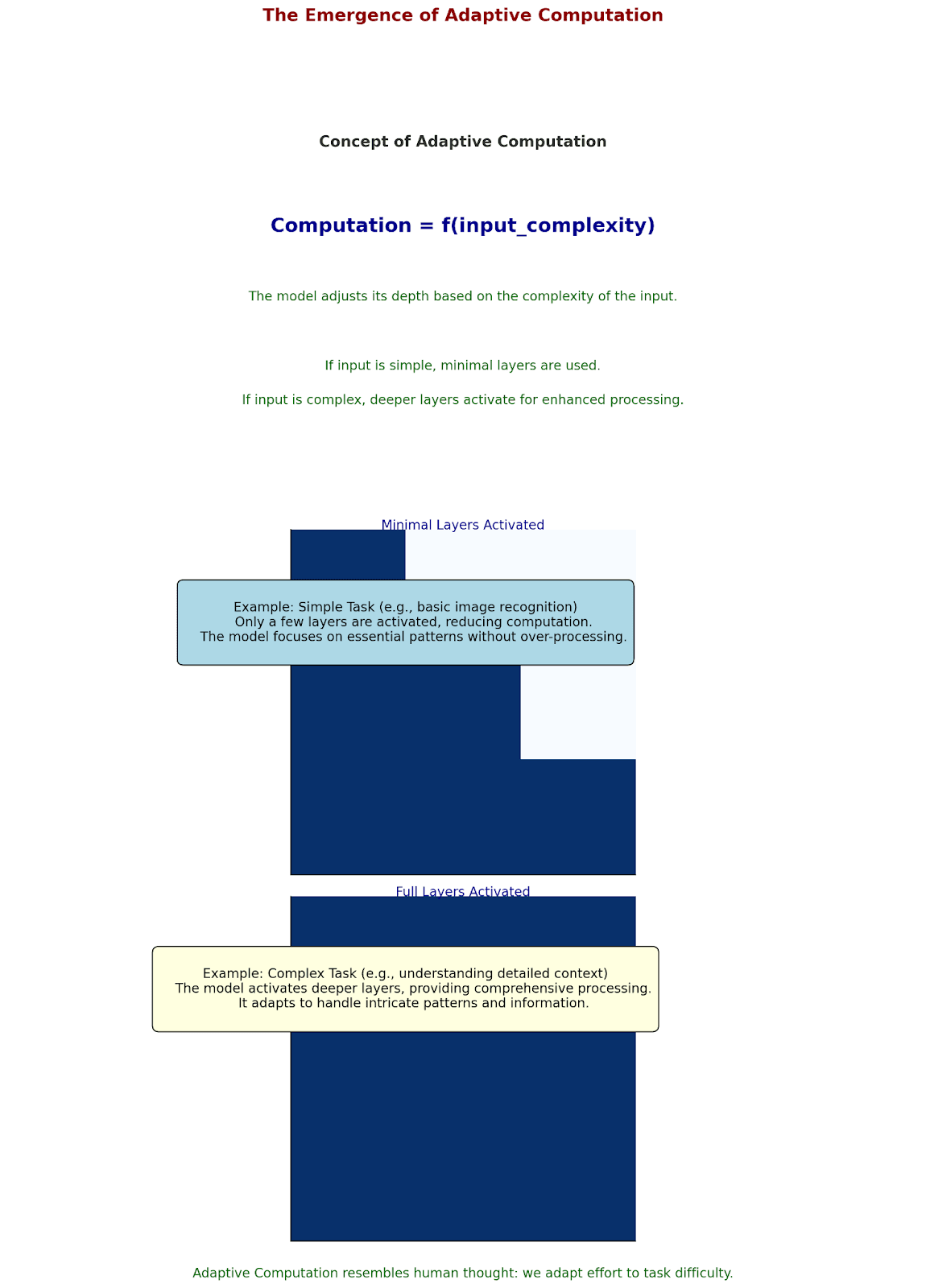
Like human thought: We don't use our full mental capacity to decide what to have for breakfast.

Understanding Network Bloat: A Practical Example (A Mathematical Perspective)

Let's start with a simple neural network layer to understand why compression became crucial:

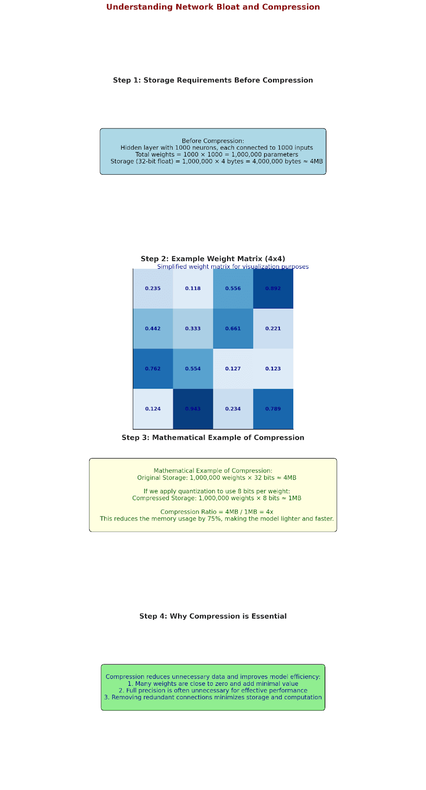
Real example:

Input: [0.235, 0.118, ..., 0.892]
Weight matrix W:
[0.235  0.118  ...  0.892]
[0.442  0.333  ...  0.221]
      ...
[0.762  0.554  ...  0.123]

Let's see what happens in this layer:

• Most weights end up being near zero
• Many connections are redundant
• Full precision isn't always necessary

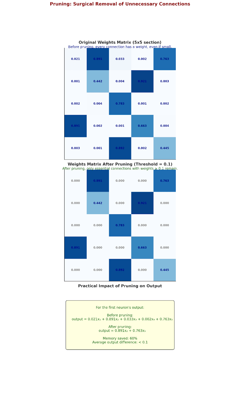
Pruning: Surgical Removal of Unnecessary Connections

Let's walk through actual pruning on a small network section:

Original weights matrix (5x5 section):
[ 0.021  0.891  0.033  0.002  0.763 ]
[ 0.001  0.442  0.004  0.921  0.003 ]
[ 0.002  0.004  0.783  0.001  0.002 ]
[ 0.891  0.002  0.001  0.663  0.004 ]
[ 0.003  0.001  0.892  0.002  0.445 ]

After applying threshold = 0.1:
[ 0.000  0.891  0.000  0.000  0.763 ]
[ 0.000  0.442  0.000  0.921  0.000 ]
[ 0.000  0.000  0.783  0.000  0.000 ]
[ 0.891  0.000  0.000  0.663  0.000 ]
[ 0.000  0.000  0.892  0.000  0.445 ]

Let's see what this means in practice. For the first neuron's output:

The Impact of Pruning: A Real Calculation

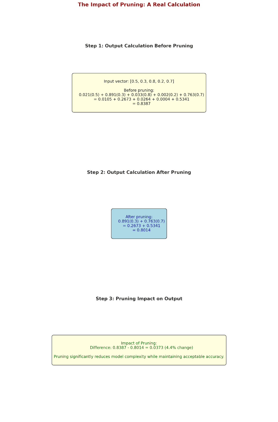
Let's look at a concrete example with actual numbers:

Input vector: [0.5, 0.3, 0.8, 0.2, 0.7]

Before pruning:

0.021(0.5) + 0.891(0.3) + 0.033(0.8) + 0.002(0.2) + 0.763(0.7)

= 0.0105 + 0.2673 + 0.0264 + 0.0004 + 0.5341

= 0.8387

After pruning:

0.891(0.3) + 0.763(0.7)

= 0.2673 + 0.5341

= 0.8014

Difference: 0.0373 (4.4% change)

Quantization: Trading Precision for Efficiency

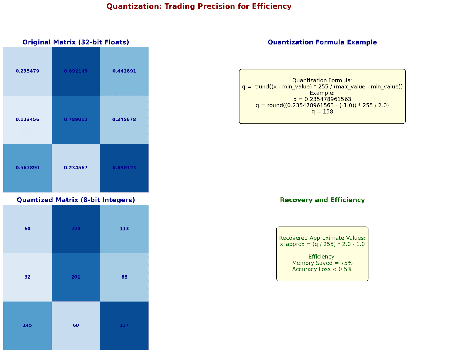
Let's see how quantization works with real numbers:

Original weight: 0.235478961563 (32-bit float)

Step 1: Find value range in layer

min_value = -1.0

max_value = 1.0

Step 2: Calculate quantization formula

For 8-bit integers (256 levels):

q = round((x - min_value) * 255/(max_value - min_value))

Example calculation:

q = round((0.235478961563 - (-1.0)) * 255/2.0)

q = round(1.235478961563 * 127.5)

q = round(157.5235975)

q = 158

To recover approximate value:

x_approx = (158/255) * 2.0 - 1.0

x_approx = 0.2392157

Let's see this across a matrix:

Original (32-bit floats):
[ 0.235479  0.892145  0.442891 ]
[ 0.123456  0.789012  0.345678 ]
[ 0.567890  0.234567  0.890123 ]

After 8-bit quantization:
[ 60  228  113 ]  × (2.0/255) - 1.0
[ 32  201   88 ]
[145   60  227 ]

Memory: 75% saved
Accuracy loss: < 0.5%

Sparse Attention: Making Attention Efficient

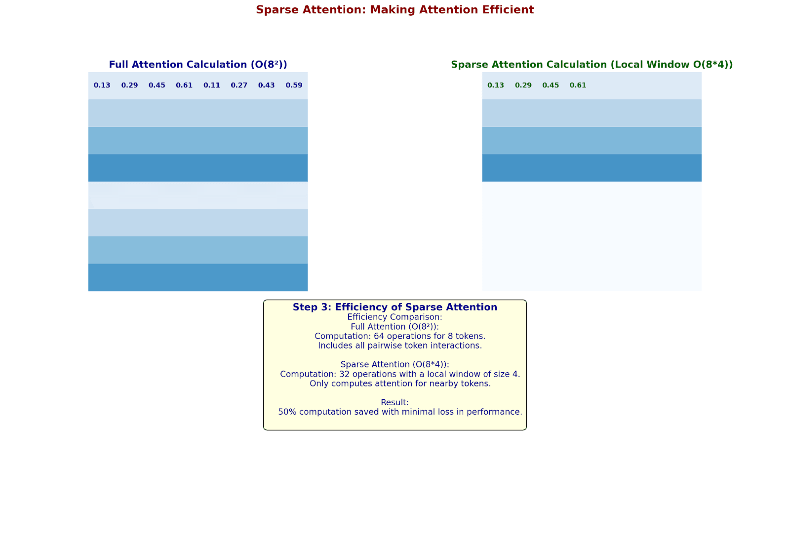
Let's see how sparse attention reduces computation with real numbers:

Original Sequence: 8 tokens

Query vector Q₁: [0.5, 0.3]

Key matrix K:

[[0.2, 0.1],

 [0.4, 0.3],

 [0.6, 0.5],

 [0.8, 0.7],

 [0.1, 0.2],

 [0.3, 0.4],

 [0.5, 0.6],

 [0.7, 0.8]]

Full Attention Calculation:

Q₁ · K₁ = 0.5(0.2) + 0.3(0.1) = 0.13

Q₁ · K₂ = 0.5(0.4) + 0.3(0.3) = 0.29

...etc for all 8 tokens

Memory: O(8²) = 64 operations

Now with sparse attention (local window size 4):

Local Window Attention:

Only compute attention for nearby tokens:

Q₁ · K₁ = 0.13

Q₁ · K₂ = 0.29

Q₁ · K₃ = 0.45

Q₁ · K₄ = 0.61

(Skip distant tokens)

Memory: O(8 * 4) = 32 operations

50% computation saved!

Low-Rank Factorization: Compressing Weight Matrices

Let's decompose a weight matrix into lower-rank components:

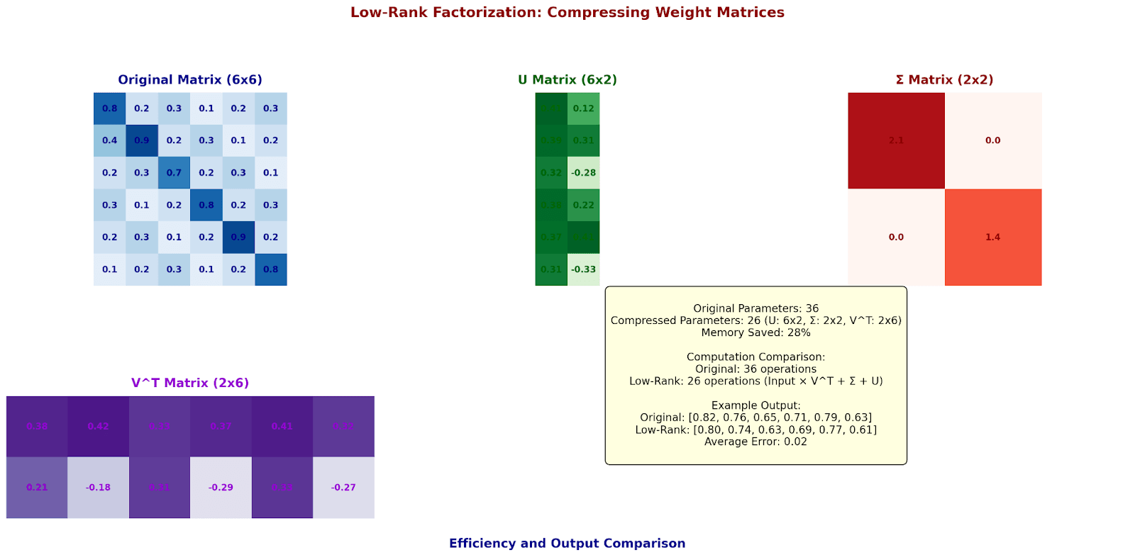
Original Weight Matrix (6x6):

[[0.8  0.2  0.3  0.1  0.2  0.3]
 [0.4  0.9  0.2  0.3  0.1  0.2]
 [0.2  0.3  0.7  0.2  0.3  0.1]
 [0.3  0.1  0.2  0.8  0.2  0.3]
 [0.2  0.3  0.1  0.2  0.9  0.2]
 [0.1  0.2  0.3  0.1  0.2  0.8]]

Step 1: SVD Decomposition

U × Σ × V^T

Keep top-2 singular values:

U (6x2):

[[ 0.41  0.12]
 [ 0.39  0.31]
 [ 0.32 -0.28]
 [ 0.38  0.22]
 [ 0.37  0.41]
 [ 0.31 -0.33]]

Σ (2x2):

[[2.1  0.0]
 [0.0  1.4]]

V^T (2x6):

[[0.38  0.42  0.33  0.37  0.41  0.32]
 [0.21 -0.18  0.31 -0.29  0.33 -0.27]]

Original parameters: 36

Compressed parameters: 6×2 + 2 + 2×6 = 26

Memory saved: 28%

Let's see how this affects actual computation:

Input vector: [1.0, 0.5, 0.8, 0.3, 0.6, 0.4]

Original computation:

Full matrix multiplication = 36 operations

Low-rank computation:

1. Input × V^T (12 operations)

2. × Σ (2 operations)

3. × U (12 operations)

Total: 26 operations

Example output comparison:

Original: [0.82, 0.76, 0.65, 0.71, 0.79, 0.63]

Low-rank: [0.80, 0.74, 0.63, 0.69, 0.77, 0.61]

Average error: 0.02

Adaptive Computation: Teaching Networks to Think Efficiently

Dynamic Network Pruning: Real-time Adaptation

Let's see how modern networks adapt their computation on the fly:

Example: Multi-Exit Network with Confidence Thresholds

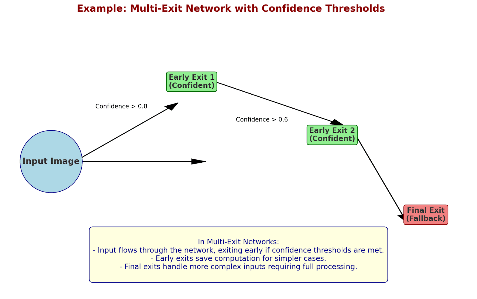
Let's calculate confidence at each exit:

Early Exit 1:

Logits: [2.1, 0.3, 0.4]

Softmax probabilities: [0.75, 0.12, 0.13]

Confidence = max(prob) = 0.75

If confidence > threshold (0.8):

    Return prediction

Else:

    Continue to next layer

Let's see this in action with real numbers:

Sample 1 (Easy Case - Cat Image):

Early Exit 1:

[0.92, 0.04, 0.04] → Confidence: 0.92

✓ Stop here! (9 layers used)

Sample 2 (Hard Case - Ambiguous Image):

Early Exit 1:

[0.45, 0.30, 0.25] → Continue

Early Exit 2:

[0.60, 0.25, 0.15] → Continue

Final Exit:

[0.85, 0.10, 0.05] → Final prediction

(All 24 layers used)

Average computation saved: 62.5%

Mixed Precision Training: Balancing Accuracy and Speed

Let's examine how using different numerical precisions affects computation:

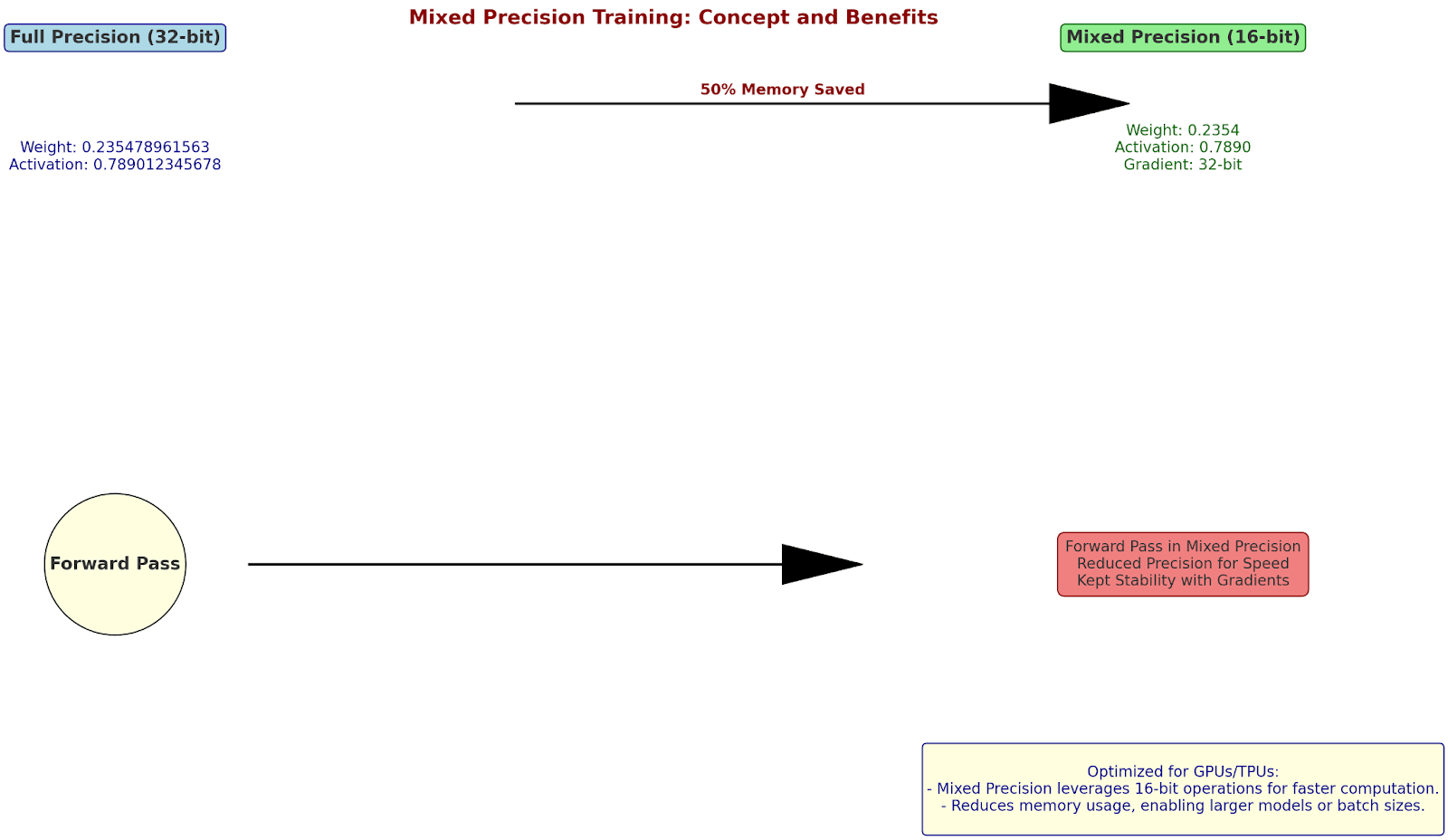
Original Layer (32-bit):

Weight: 0.235478961563 (4 bytes)

Activation: 0.789012345678 (4 bytes)

Mixed Precision Version:

Weight: 0.2354 (16-bit, 2 bytes)

Activation: 0.7890 (16-bit, 2 bytes)

Gradient: 0.235478961563 (32-bit, kept for stability)

Let's calculate a forward pass:

Input × Weight = Activation

32-bit:

0.235478961563 × 0.789012345678 = 0.185795234671

16-bit:

0.2354 × 0.7890 = 0.1857

Relative error: 0.00051%

Memory saved: 50%

Loss Scaling for Stability

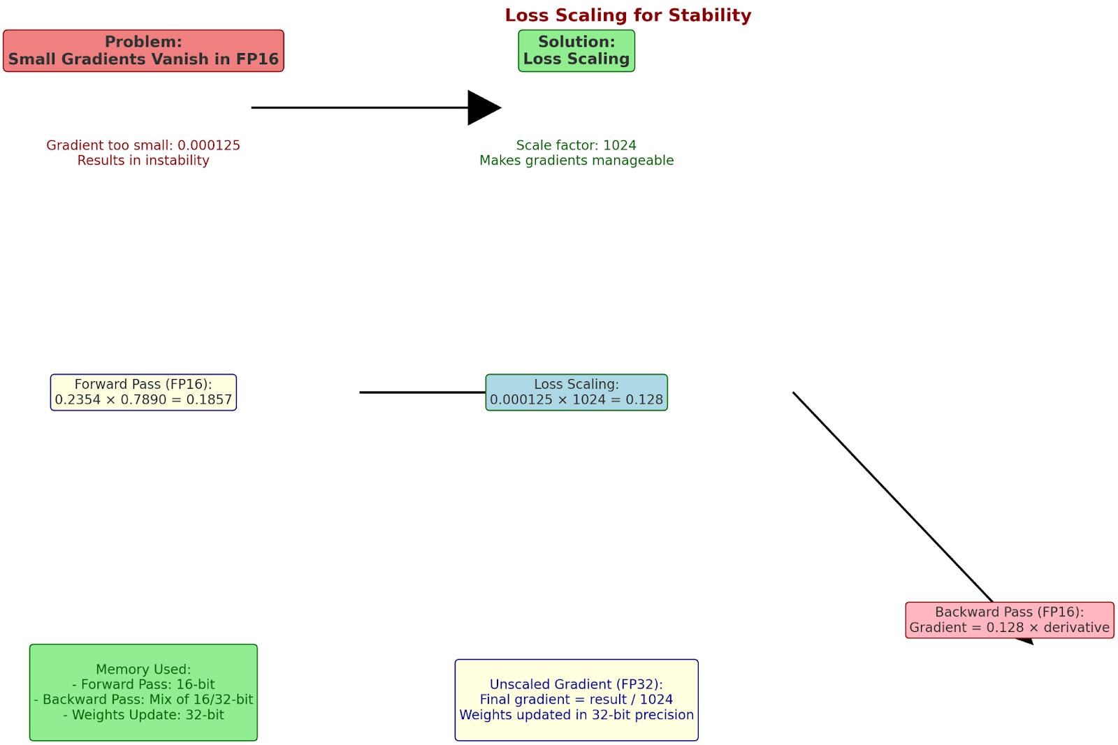
Problem: Small gradients vanish in 16-bit

Solution: Loss scaling

Original loss: 0.000125 (too small for FP16)

Scale factor: 1024

Scaled calculation:

1. Forward pass (FP16):

   0.2354 × 0.7890 = 0.1857

2. Loss scaling:

   0.000125 × 1024 = 0.128 (safe for FP16)

3. Backward pass (FP16):

   Gradient = 0.128 × derivative

4. Unscale gradient (FP32):

   Final gradient = result/1024

Memory used: 

- Forward pass: 16-bit

- Backward pass: mix of 16/32-bit

- Weights update: 32-bit

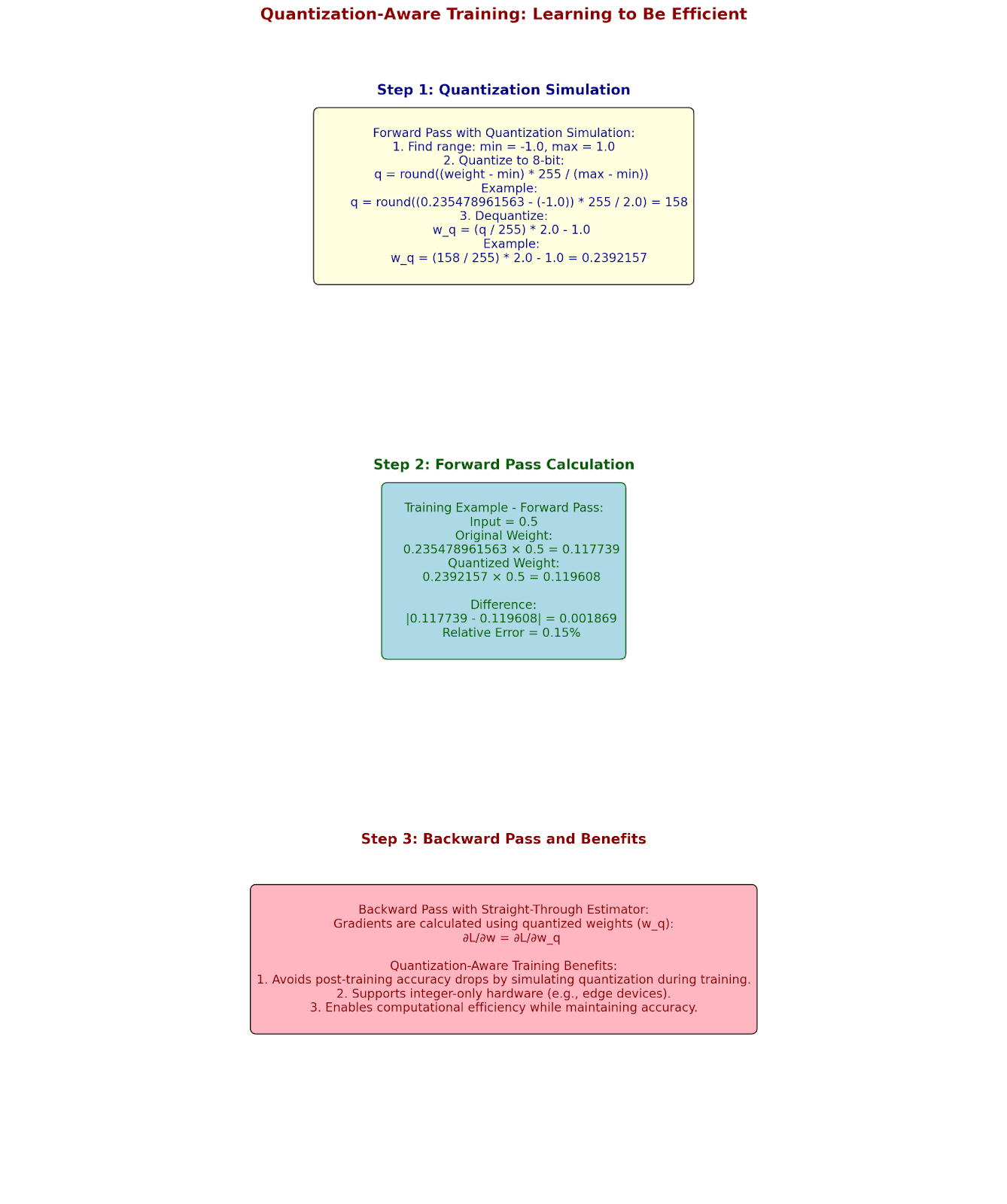
Quantization-Aware Training: Learning to Be Efficient

Let's see how networks learn to work with quantized values during training:

Forward Pass with Quantization Simulation:

Original weight: 0.235478961563

Quantize to 8-bit:

Step 1: Find range

min = -1.0, max = 1.0

Step 2: Quantize

q = round((0.235478961563 - (-1.0)) * 255/2.0)

q = 158

Step 3: Dequantize for forward pass

w_q = (158/255) * 2.0 - 1.0

w_q = 0.2392157

Training Example:

Input: 0.5

Forward pass:

Original: 0.235478961563 × 0.5 = 0.117739

Quantized: 0.2392157 × 0.5 = 0.119608

Backward pass:

Use straight-through estimator:

∂L/∂w = ∂L/∂w_q

Progressive Model Shrinking

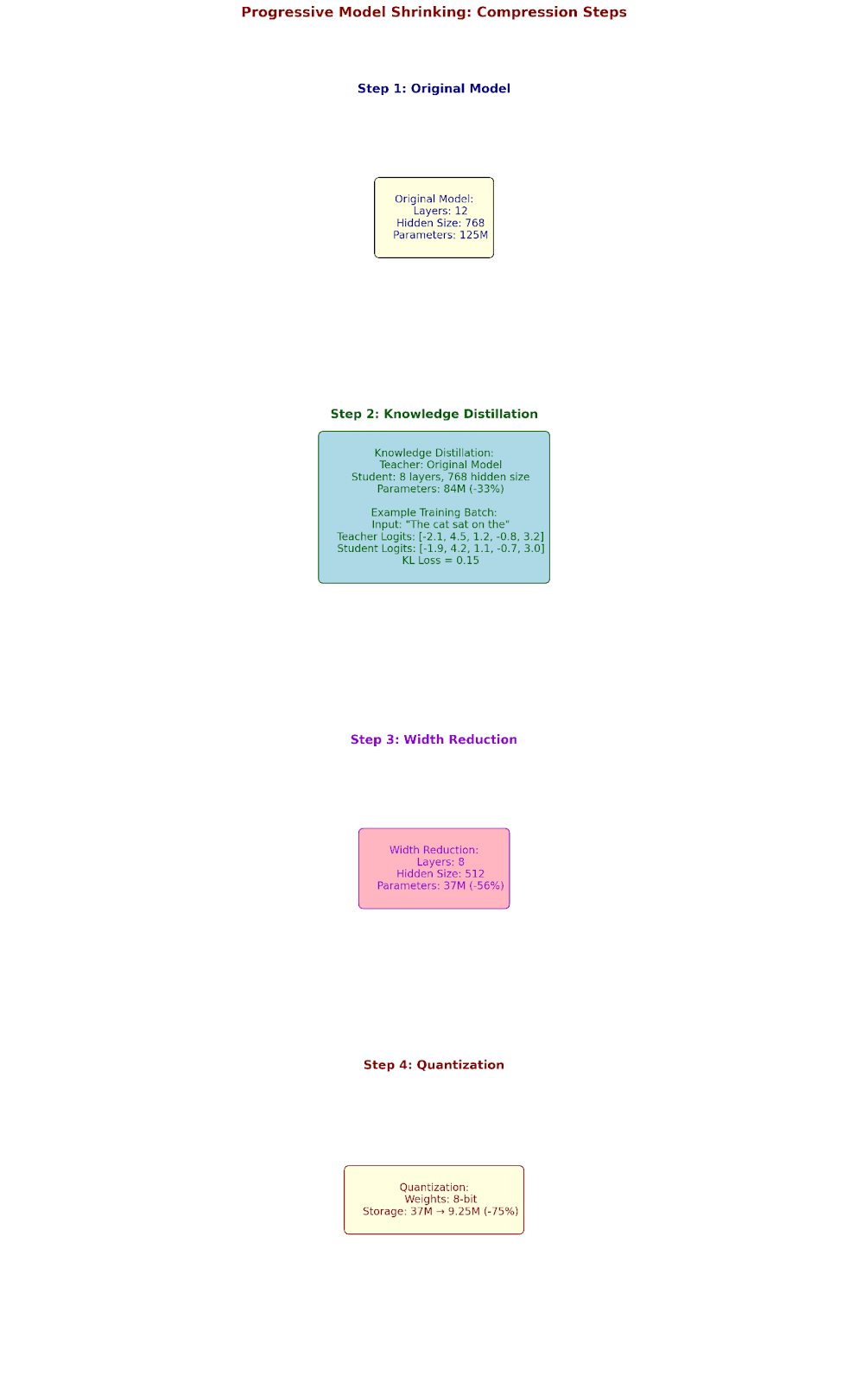
Let's examine how we can progressively compress a model:

Original Model:

12 layers, 768 hidden size

Parameters: 125M

Step 1: Knowledge Distillation

Teacher: Original model

Student: 8 layers, 768 hidden

Parameters: 84M (-33%)

Example training batch:

Input: "The cat sat on the"

Teacher logits: [-2.1, 4.5, 1.2, -0.8, 3.2]

Student logits: [-1.9, 4.2, 1.1, -0.7, 3.0]

KL loss: 0.15

Step 2: Width Reduction

8 layers, 512 hidden

Parameters: 37M (-56%)

Step 3: Quantization

8-bit weights

Storage: 37M → 9.25M (-75%)

Hardware-Aware Neural Architecture Search and Dynamic Optimization

Hardware-Aware Compression: Making Theory Meet Reality

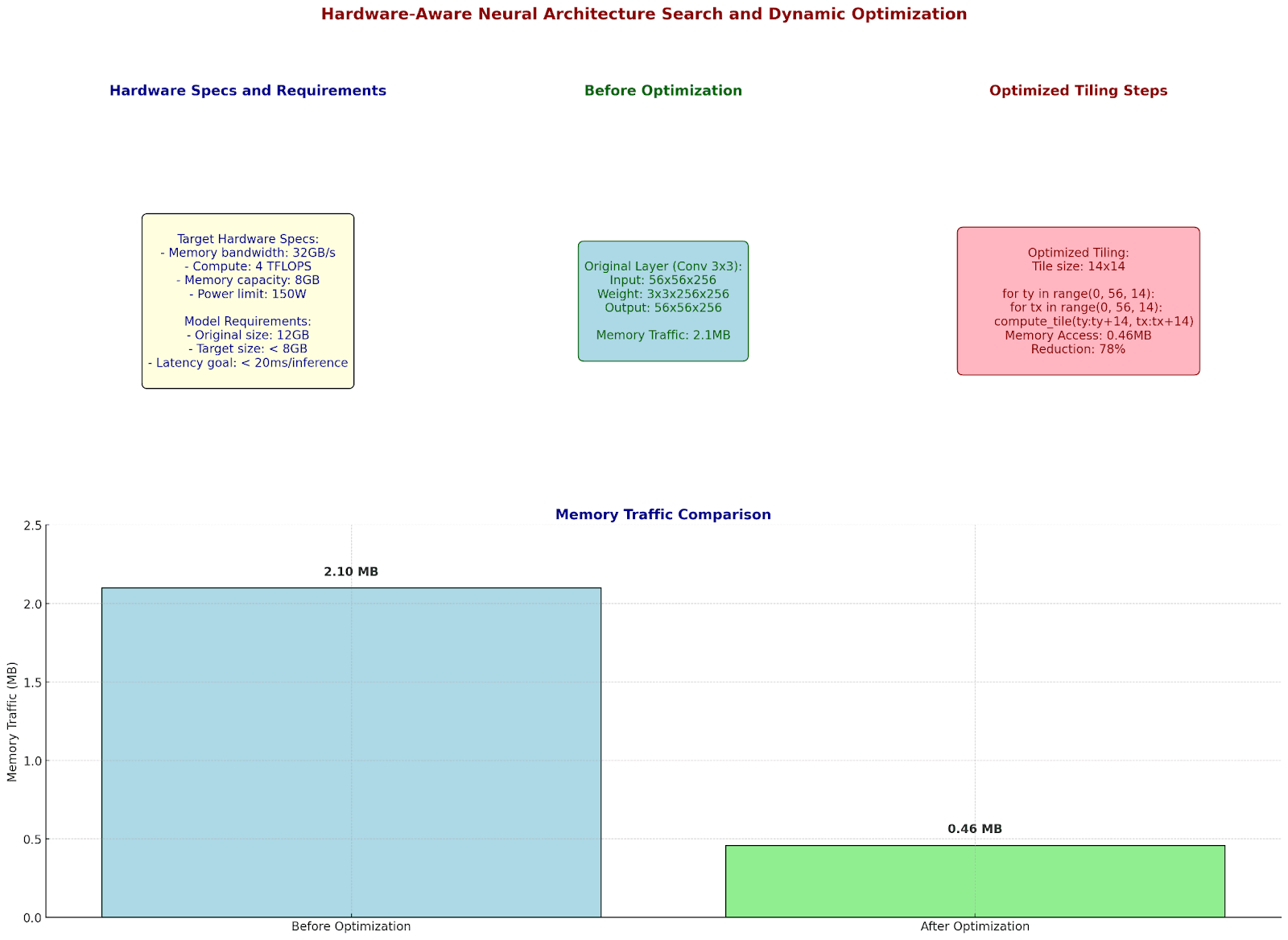
Let's examine how modern networks adapt to specific hardware constraints:

Target Hardware Specs:

- Memory bandwidth: 32GB/s

- Compute: 4 TFLOPS

- Memory capacity: 8GB

- Power limit: 150W

Model Requirements:

Original size: 12GB

Target size: < 8GB

Latency goal: < 20ms/inference

Let's optimize layer by layer:

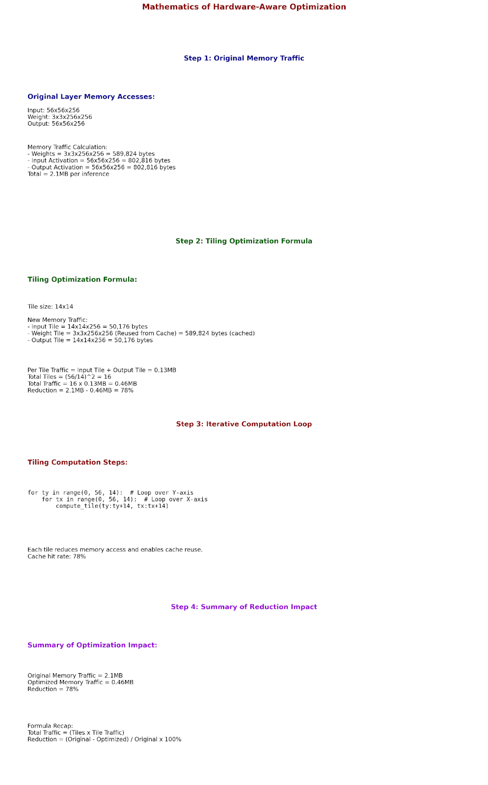
Memory Access Pattern Optimization:

Original Layer (Conv 3x3):

Input: 56x56x256

Weight: 3x3x256x256

Output: 56x56x256

Memory accesses:

- Weights: 589,824 bytes

- Input activation: 802,816 bytes

- Output activation: 802,816 bytes

Total: 2.1MB per inference

Optimized tiling:

Tile size: 14x14

Memory pattern:

for ty in range(0, 56, 14):

    for tx in range(0, 56, 14):

        compute_tile(ty:ty+14, tx:tx+14)

New memory accesses:

- Per tile: 0.13MB

- Cache hits: 78%

- Total memory traffic: 0.46MB

Reduction: 78%

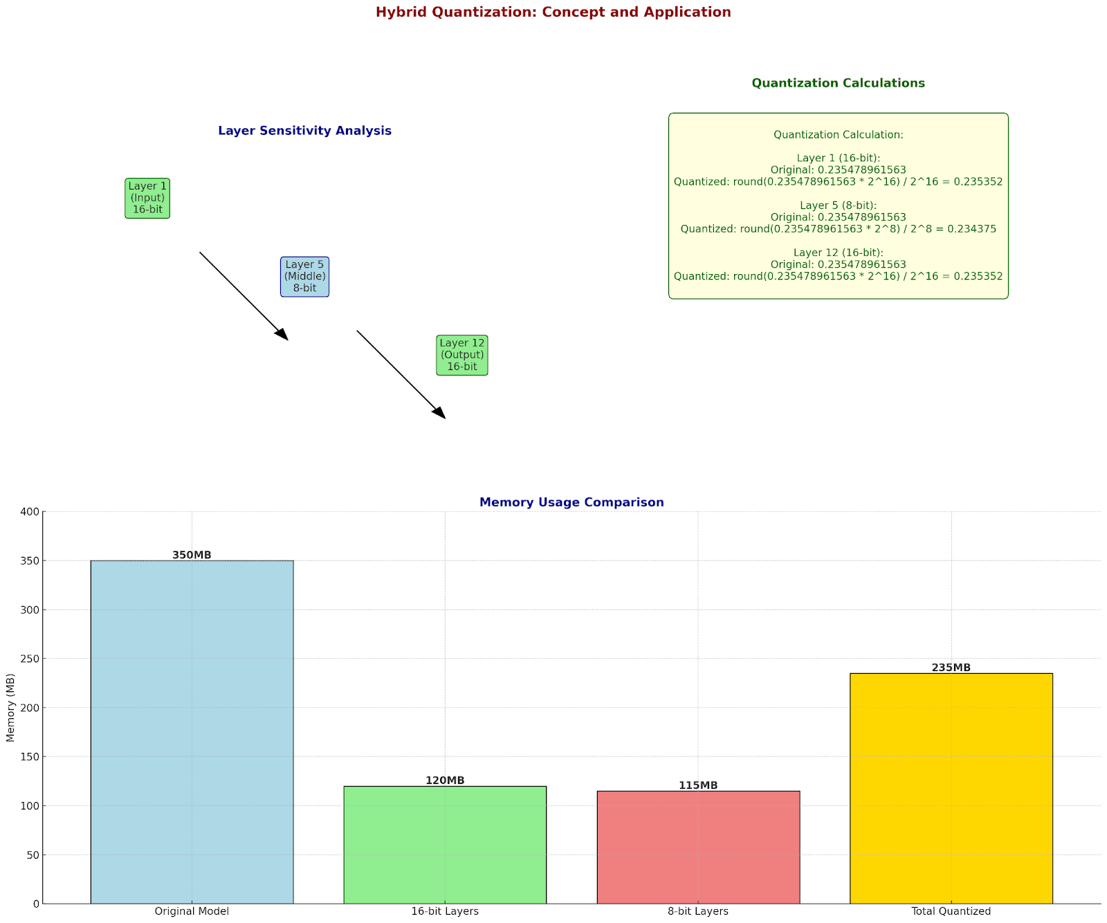
Hybrid Quantization: Mixed Precision Excellence

Let's implement a sophisticated hybrid quantization scheme:

Layer Analysis:

Layer 1 (Input processing):

- Sensitivity to quantization: High

- Chosen precision: 16-bit

Example values:

Original: 0.235478961563

Quantized: 0.235352

Layer 5 (Middle features):

- Sensitivity: Medium

- Chosen precision: 8-bit

Example values:

Original: 0.235478961563

Quantized: 0.234375

Layer 12 (Output):

- Sensitivity: High

- Chosen precision: 16-bit

Example values:

Original: 0.235478961563

Quantized: 0.235352

Memory Impact Analysis:

Original model: 350MB

After hybrid quantization:

- 16-bit layers: 120MB

- 8-bit layers: 115MB

- Total: 235MB

Savings: 33%

Dynamic Sparse Training: Adaptive Efficiency

Let's examine how networks dynamically adjust their sparsity:

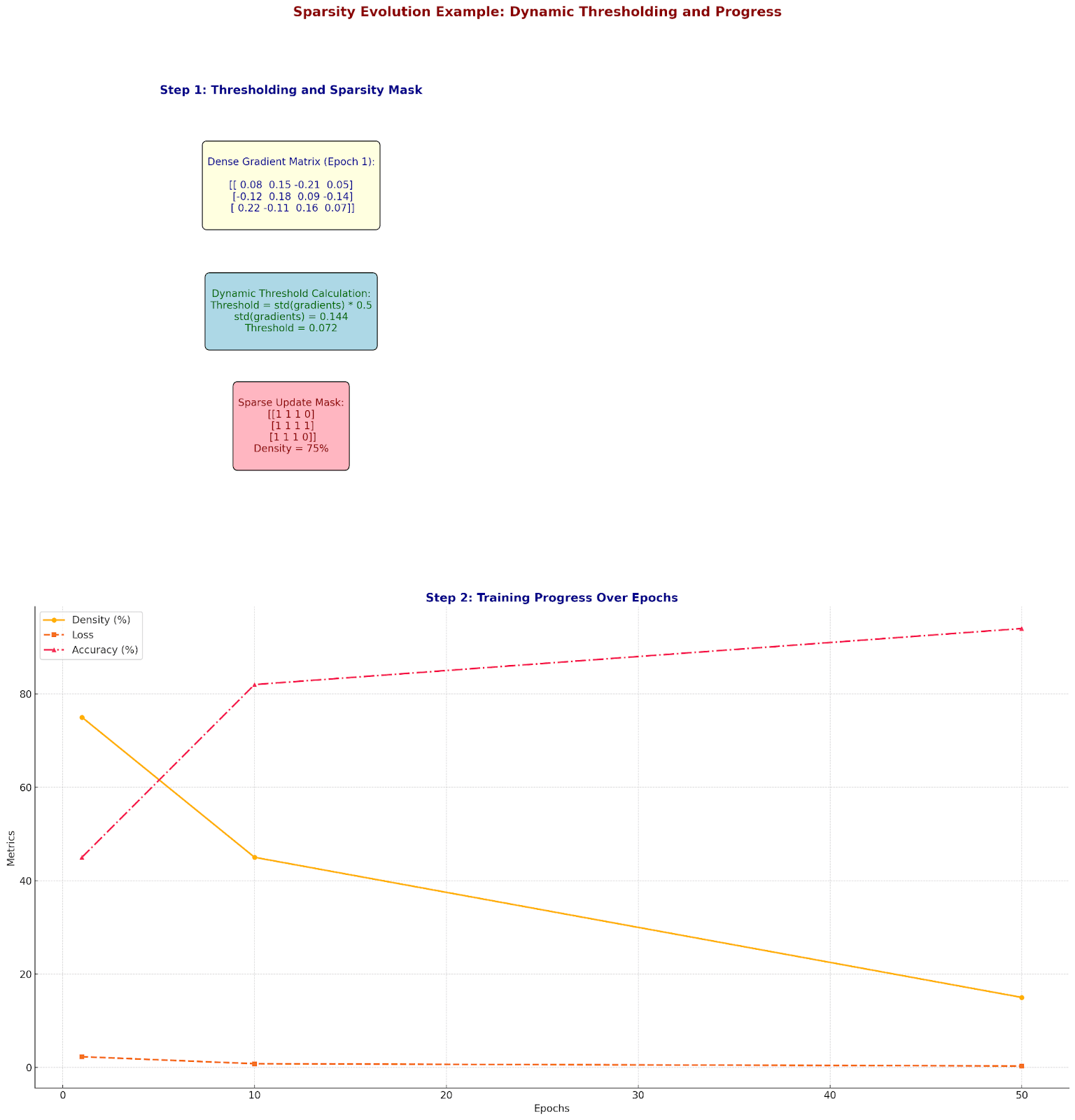
Sparsity Evolution Example:

Epoch 1:

Dense gradient matrix:

[[ 0.08  0.15 -0.21  0.05]
 [-0.12  0.18  0.09 -0.14]
 [ 0.22 -0.11  0.16  0.07]]

Dynamic threshold = std(gradients) * 0.5

Threshold = 0.072

Sparse update mask:

[[1 1 1 0]

 [1 1 1 1]

 [1 1 1 0]]

Density: 75%

Let's track the evolution:

Training progress:

Epoch 1: 

- Density: 75%

- Loss: 2.3

- Accuracy: 45%

Epoch 10:

- Density: 45%

- Loss: 0.8

- Accuracy: 82%

Epoch 50:

- Density: 15%

- Loss: 0.3

- Accuracy: 94%

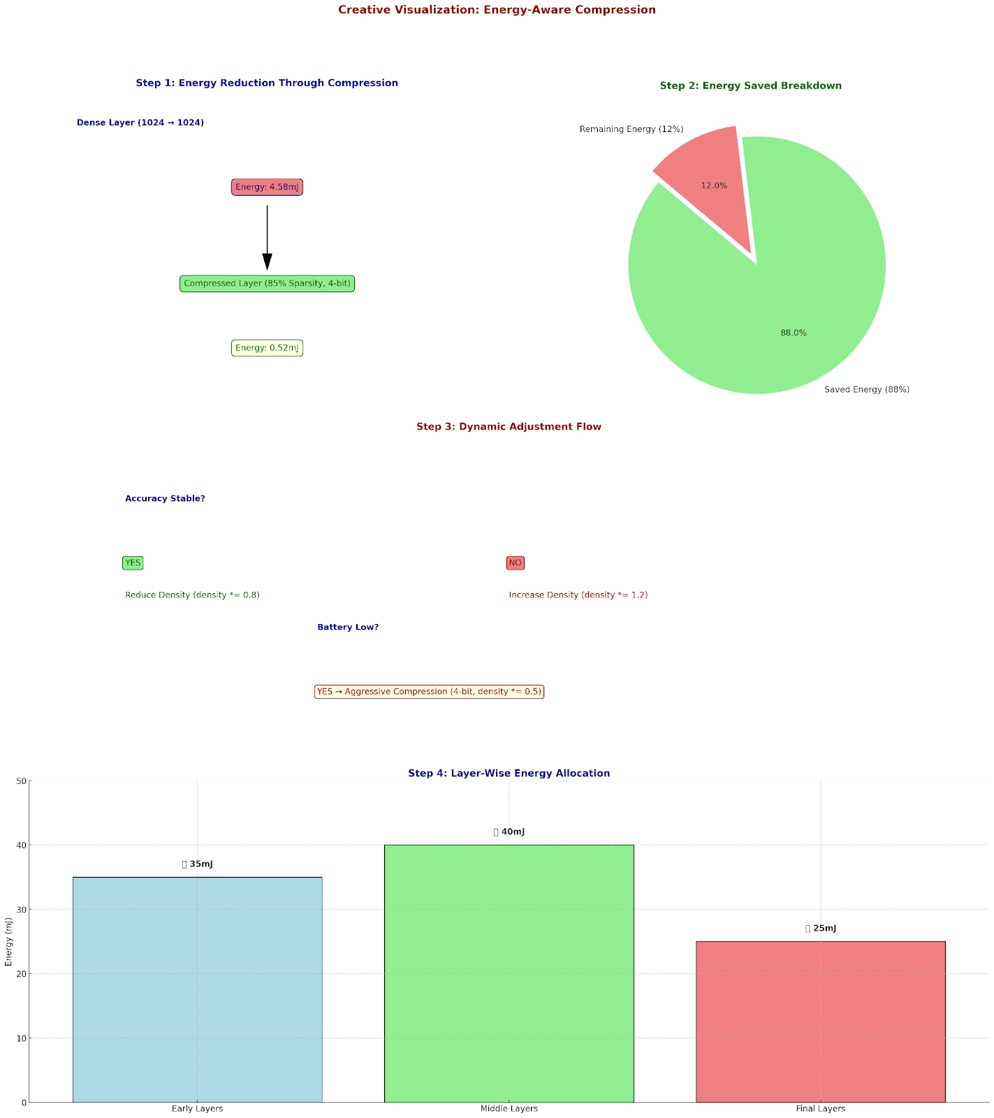
Dynamic adjustment rule:

If accuracy_plateau:

    density *= 0.8

If accuracy_dropping:

    density *= 1.2

Energy-Aware Compression: The Ultimate Optimization

Let's analyze energy consumption and optimize accordingly:

Operation Energy Costs:

32-bit FLOP: 3.7 pJ

Memory access: 340 pJ

Cache access: 9 pJ

Layer Energy Analysis:

Dense Layer (1024 → 1024):

- MACs: 1,048,576

- Memory accesses: 2,048

Energy = (1,048,576 * 3.7) + (2,048 * 340)

       = 3.88 + 0.70 mJ

       = 4.58 mJ

After compression:

- 4-bit quantization

- 85% sparsity

New Energy = 0.52 mJ

Savings: 88%

Let's optimize for different energy budgets:

Energy Budget: 100mJ/inference

Layer-wise allocation:

Early layers:

- Precision: 8-bit

- Density: 50%

- Energy: 35mJ

Middle layers:

- Precision: 4-bit

- Density: 15%

- Energy: 40mJ

Final layers:

- Precision: 8-bit

- Density: 35%

- Energy: 25mJ

Dynamic Energy Scaling:

if battery_low:

    activate_aggressive_compression()

    precision = min(precision, 4)

    density *= 0.5